Updated May 11, 2023
Gradient Descent in Machine Learning:- A Basic Introduction
Gradient Descent is an optimization algorithm used in machine learning models to find the minimum value of a cost function. It does this by taking small steps in the direction that is opposite to the gradient of the cost function until it reaches a local minimum. The learning rate determines the size of each step and can be adjusted to balance convergence speed and accuracy. Stochastic Gradient Descent is a variation of the algorithm that randomly selects samples to compute the gradient, making it faster but less precise.
Key Takeaways
- The cost function must be differentiable for Gradient Descent to work.
- It can coincide with a local minimum instead of the global minimum.
- Choosing an appropriate learning rate can be challenging and requires experimentation.
- Gradient Descent can be sensitive to initial parameter values.
- Variations of Gradient Descent, including Mini-Batch Gradient Descent and Adaptive Moment Estimation, can improve its performance in specific scenarios.
History of Gradient Descent
The idea of Gradient Descent dates back to the early 19th century when Carl Friedrich Gauss proposed the method of least squares for fitting a linear model to data. The concept was later extended by Leonhard Euler and Joseph-Louis Lagrange, who introduced the method of steepest descent for finding the minimum of a function. In modern times, Gradient Descent was popularised by the machine learning community in the 20th century, with the first work being done by Arthur Samuel in the 1950s. Today, it remains a fundamental building block in many machine learning algorithms, including deep neural networks.
The algorithm works by iteratively taking small steps in the direction that is opposite to the gradient of the cost function, with the learning rate controlling the size of each step.
By doing so, it gradually converges to a local minimum of the cost function, which corresponds to the optimal model parameters. While simple in concept, Gradient Descent can be challenging to implement effective due to issues such as sensitivity to initial parameter values, local optima, and choice of learning rate. Nonetheless, it remains a powerful and widely used algorithm in the field of machine learning.
Defining Local Minimum and Maximum
Local Minimum
In mathematics and machine learning, a local minimum is a point in a function where the value of the function is less than all nearby points, but it may not be the global minimum over the entire domain of the function. To identify a local minimum, one needs to find the critical points of the function where its derivative is zero and examine the curvature of the function at these points. If the function is concave upwards at a critical point, it is a local minimum. This concept is essential in optimization and can arise in many machine learning applications.
Local Maximum
In mathematics and machine learning, a local maximum refers to a point in a function where the value of the function is greater than all nearby points, but it may not be the global maximum over the entire domain of the function. A local maximum can be identified by finding the critical points of the function, where its derivative is zero, and checking the concavity of the function at these points. If the function is concave downwards at a critical point, it is a local maximum. This concept is important in optimization and can arise in various machine-learning applications.
Working of Gradient Descent in Machine Learning
Suppose we have a simple linear regression model that predicts the price of a house based on its size. The model can be represented by the following equation: y = mx + b, where y is the price of the house, x is its size, m is the slope of the line, and b is the intercept. We can use Gradient Descent to find the optimal values of m and b that minimize the mean squared error between the predicted and actual prices of the houses in our dataset.
The goal of Gradient Descent is to find the optimal values of m and b that minimize the cross-entropy loss function between the predicted and actual probabilities of admission in our dataset.
The steps involved in Gradient Descent are as follows:
- Initialize the values of m and b to random values.
- Calculate the predicted values of y using the current values of m and b.
- Calculate the mean squared error between the predicted and actual values of y.
- Calculate the partial derivatives of the cost function with respect to m and b.
- Update the values of m and b using the partial derivatives and a learning rate, which determines the size of the step taken in the direction of the steepest descent.
- Repeat steps 2-5 until the cost function converges to a minimum.
For example, let’s say we have a dataset of 10 houses with their sizes and prices:
(1000, 40000), (2000, 80000), (3000, 120000), (4000, 160000), (5000, 200000), (6000, 240000), (7000, 280000), (8000, 320000), (9000, 360000), (10000, 400000)
Using Gradient Descent, we can update the values of m and b iteratively until we find the best-fit line that minimizes the mean squared error. The learning rate determines the size of the step taken in each iteration.
By updating the values of m and b using the partial derivatives of the cost function, we gradually converge to the optimal values that minimize the mean squared error. Once we reach the minimum, we stop updating the values of m and b and use the resulting model to predict the prices of new houses based on their size.
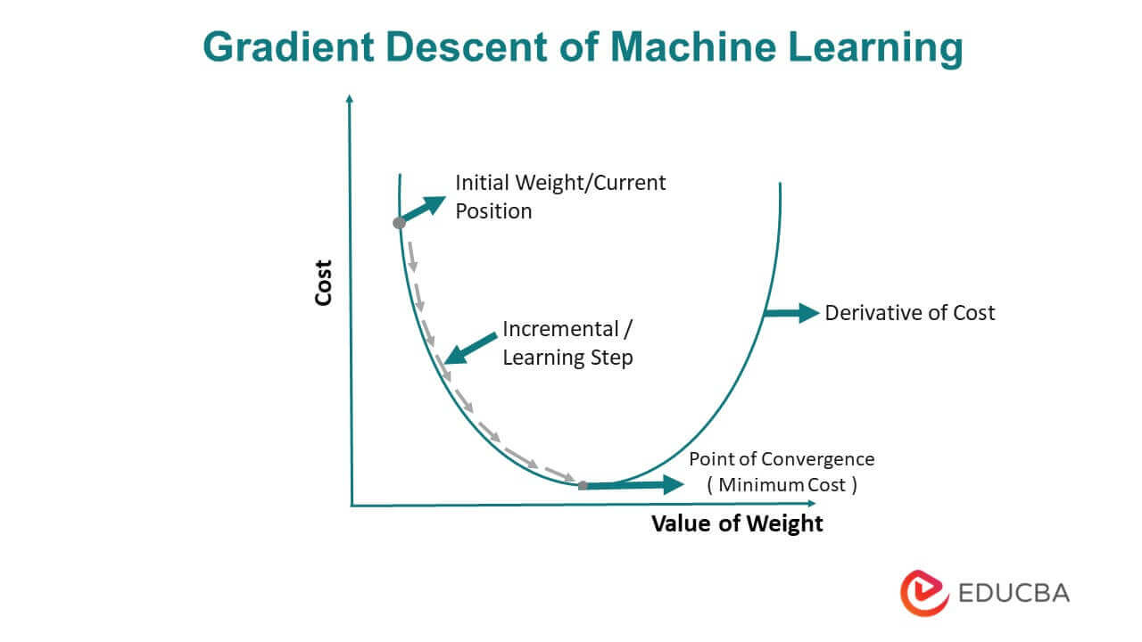
IMAGE OF GRADIENT DESCENT
Point of Convergence: “Point of convergence” refers to the point in the optimization process where the algorithm has minimized the cost function as much as possible and reached a minimum value or converged at a stable point. At this point, further iterations of the algorithm will not lead to significant improvements in the model’s performance.
The algorithm works by computing the gradient of the cost function with respect to the model parameters, which indicates the direction of the steepest ascent. To minimize the cost function, the algorithm updates the model parameters in the opposite direction of the gradient, taking a small step determined by the learning rate. This process is repeated until the algorithm converges to a minimum of the cost function.
Learning Rate: The learning rate is a hyperparameter that establishes how much the model’s parameters are modified in response to the cost function gradient; it also regulates the size during each iteration of an optimization technique like gradient descent.
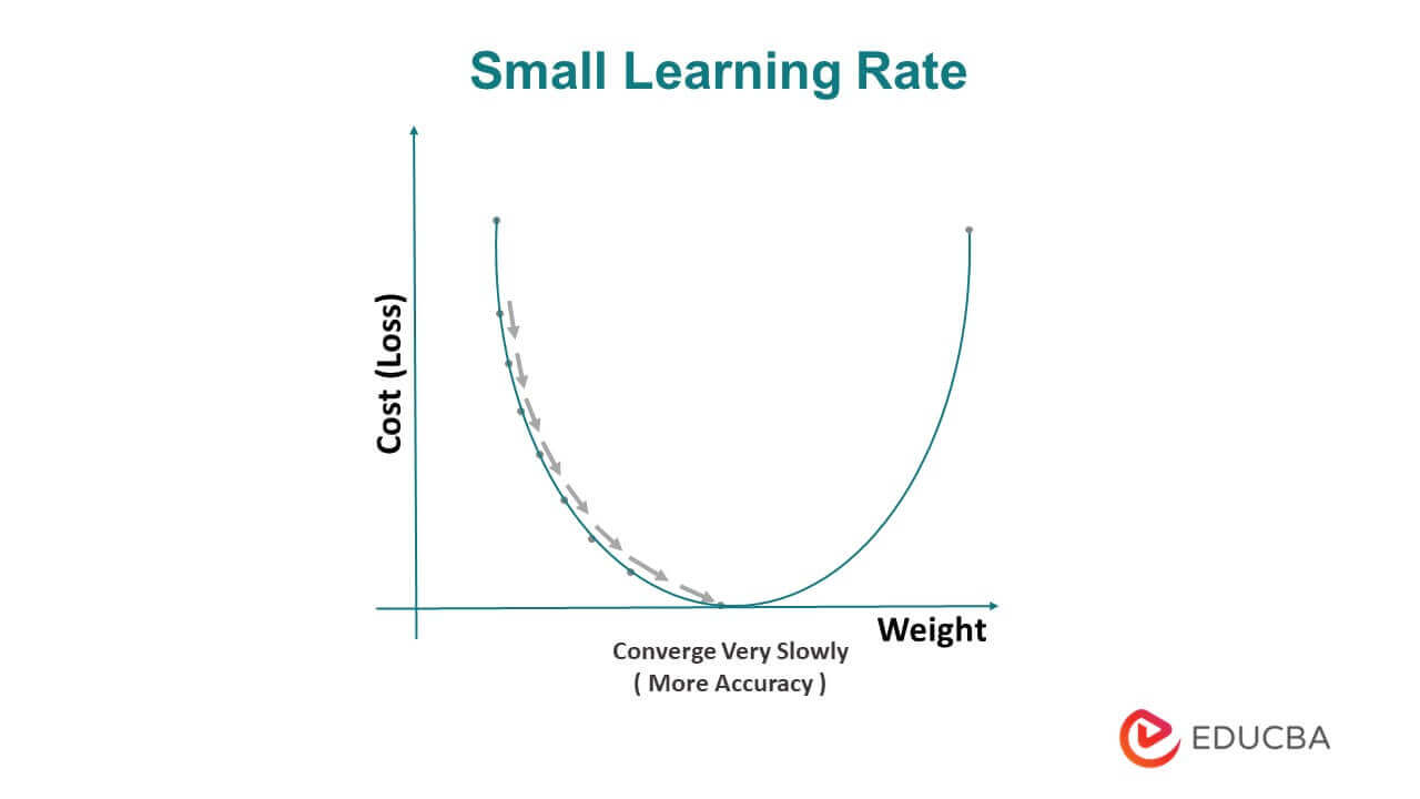
A small learning rate refers to a relatively low value used to update the model’s parameters during the optimization process. A small learning rate leads to slower convergence.
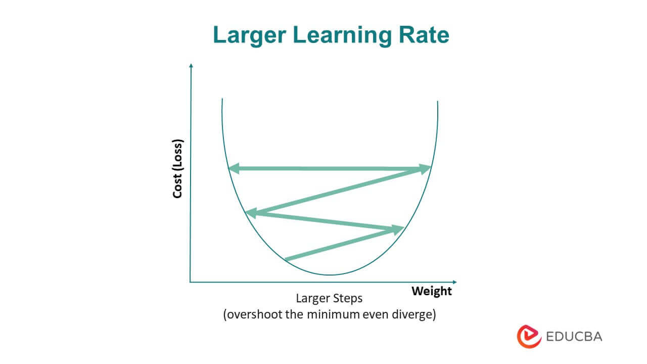
On the other hand, a big learning rate refers to a relatively high value used to update the model’s parameters. The learning rate determines the step size taken toward the optimal solution during gradient descent. A large learning rate can result in overshooting the minimum and unstable convergence.
Large Learning Rate
Small Learning Rate
The choice of the learning rate is important in Gradient Descent as a high learning rate can cause the algorithm to overshoot the minimum and oscillate, while a low learning rate can lead to slow convergence. Variations of Gradient Descent, such as Stochastic Gradient Descent and Mini-Batch Gradient Descent, can improve its performance. Stochastic Gradient Descent randomly samples a subset of the training data to compute the gradient, which makes it faster but noisier. Mini-Batch Gradient Descent computes the gradient on a small batch of samples, which balances convergence speed and accuracy. Overall, Gradient Descent is a fundamental building block in many machine learning algorithms and is used extensively in deep learning.
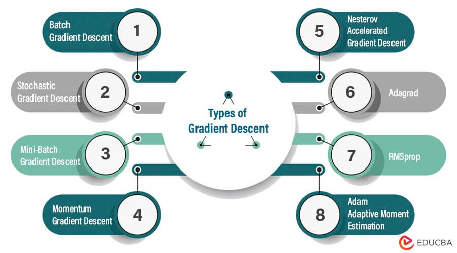
Types of Gradient Descent
1. Batch Gradient Descent: This is the simplest form of Gradient Descent, where the gradient of the cost function is calculated using the entire training set. The model parameters are then updated based on this calculated gradient. Batch Gradient Descent is slow and computationally expensive but is guaranteed to converge to the global minimum if the cost function is convex.
2. Stochastic Gradient Descent (SGD): SGD updates the model parameters after processing each training sample, using a single sample or a small batch of samples to compute the gradient. This approach is faster and can handle large datasets better than Batch Gradient Descent. However, the learning process can be noisy, leading to slower convergence or getting stuck in local optima.
3. Mini-Batch Gradient Descent: This method computes the gradient using a small batch of training samples, which provides a balance between the accuracy of the speed of Stochastic Gradient Descent and Batch Gradient Descent. This approach can converge faster than Batch Gradient Descent and is less noisy than Stochastic Gradient Descent.
4. Momentum Gradient Descent: Momentum GD adds a momentum term to the update rule, which helps to smooth out oscillations in the gradient descent path and accelerate convergence. The momentum term accumulates the gradient updates over time and helps the algorithm to move faster in the correct direction and avoid local optima.
5. Nesterov Accelerated Gradient Descent (NAG): Nesterov’s Accelerated Gradient Descent is a modification of momentum Gradient Descent that accounts for the next step’s momentum and improves convergence speed. NAG computes the gradient of the cost function after adding the momentum term to the current position, which provides a better estimate of the gradient and improves convergence speed.
6. Adagrad: Adagrad adapts the learning rate for each model parameter based on the history of gradients for that parameter. This approach helps to converge quickly on sparse features, making it useful for natural language processing and computer vision applications.
7. RMSprop: RMSprop is a modification of Adagrad that normalizes the historical gradient sum. It helps to adapt more robustly to the changing gradient surface and prevents the learning rate from becoming too small.
8. Adam (Adaptive Moment Estimation): Adam combines the concepts of momentum and adaptive learning rates. It uses the first and second moments of the gradient to calculate the adaptive learning rate and momentum term. Adam is a popular optimization algorithm for training deep neural networks due to its effectiveness in converging quickly to the minimum.
In general, selecting the appropriate Gradient Descent algorithm depends on the specific problem, dataset size, and model complexity. It is often beneficial to experiment with multiple algorithms and tune their hyperparameters to optimize convergence speed and accuracy.
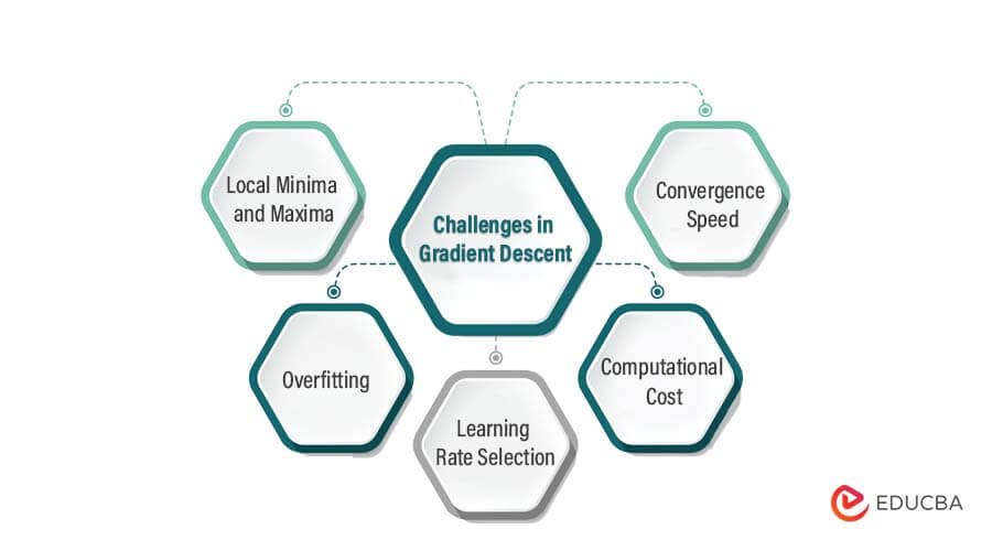
Challenges in Gradient Descent
1. Local minima and maxima: The cost function may have multiple local minima or maxima, which can cause Gradient Descent to converge to a suboptimal solution. This can be addressed using techniques such as momentum, which can help the algorithm to escape from local optima.
2. Overfitting: Gradient Descent can be prone to overfitting, where the model becomes too complex and fits the training data too closely. This can be addressed by using regularization techniques such as L1 or L2 regularization, which penalize large parameter values.
3. Learning rate selection: Selecting an appropriate learning rate can be a challenging task. When the learning rate is too high, the algorithm may overshoot the minimum and fail to converge, while a learning rate that is too low can lead to slow convergence or getting stuck in local optima. There are techniques such as learning rate decay and adaptive learning rates that can help to address this challenge.
4. Computational cost: Gradient Descent can be computationally expensive, especially for large datasets or complex models. This can be addressed by using parallel processing or by implementing more efficient algorithms, such as mini-batch Gradient Descent.
5. Convergence speed: The convergence speed of Gradient Descent can be slow, especially for high-dimensional models. This can be addressed using optimization techniques such as Nesterov Accelerated Gradient Descent, Adam, or RMSprop, which can help the algorithm to converge faster.
Tips for Working with Gradient Descent in Machine Learning
- Normalize the input data: Normalizing the input data can help Gradient Descent to converge faster and can prevent gradient explosion or vanishing.
- Choose an appropriate learning rate: The learning rate controls the step size taken in the direction of the gradient. An appropriate learning rate can help the algorithm converge faster without overshooting the minimum.
- Use a good initialization strategy: Initializing the model parameters with appropriate values can help the algorithm converge faster and avoid getting stuck in local optima.
- Use mini-batch Gradient Descent: Mini-batch Gradient Descent can provide a good balance between convergence speed and computational efficiency.
- Monitor the convergence process: Monitoring the convergence process can help to detect issues such as overfitting, underfitting, or slow convergence. This can be done by tracking the training loss or validation error over time.
- Use regularization techniques: Regularization techniques such as L1 or L2 regularization can help to avoid overfitting and enhance the generalization performance of the model.
- Choose an appropriate cost function: The cost function should be appropriate for the problem at hand and should reflect the desired model behavior. An appropriate cost function can help Gradient Descent to converge faster and can prevent the model from getting stuck in local optima.
- Experiment with different optimization algorithms: Different optimization algorithms may perform differently for different problems. Experimenting with different algorithms can help to find the one that works best for the problem at hand.
Conclusion
Gradient Descent is a widely used optimization algorithm in machine learning that helps to enhance the performance of models by reducing the cost function. Despite its limitations, being aware of its drawbacks and practical tips can aid in building more reliable and accurate models. Therefore, it is considered an effective and essential technique in the field of machine learning.
FAQs
1. What is the learning rate in Gradient Descent?
The learning rate is known as a hyperparameter that controls the size of the step taken in the direction of the negative gradient. A small learning rate results in slow convergence, while a large learning rate can cause the algorithm to overshoot the minimum and diverge.
2. What is the difference between batch, stochastic, and mini-batch Gradient Descent?
Batch Gradient Descent determines the gradient using the entire training set, while stochastic Gradient Descent computes the gradient using a single randomly chosen training example. Mini-batch Gradient Descent computes the gradient using a small random subset of the training set.
3. What is the difference between Gradient Descent and Gradient Boosting?
Gradient Descent is a widely-used optimization algorithm in machine learning that iteratively updates the parameters of a model to minimize a given cost function. In contrast, Gradient Boosting is a machine learning technique that improves the performance of decision trees by combining multiple weak learners to form a strong learner. This is done by iteratively fitting new models to the residuals of the previous model. While both Gradient Descent and Gradient Boosting have similar iterative procedures, they have different objectives and use cases.
Recommended Article
We hope that this EDUCBA information on “Gradient Descent in Machine Learning” was beneficial to you. You can view EDUCBA’s recommended articles for more information.
