Updated August 11, 2023
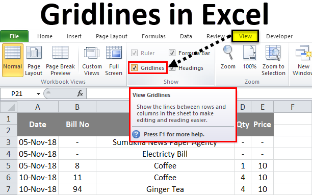
Gridlines in Excel
Gridlines in Excel can be activated from the Excel Option’s Advanced tab. Therefrom, the Display option for the worksheet, check the box of Gridlines. We can also select the color of the gridlines we want in Excel worksheets. Once we print the sheet or see the print preview of any worksheet, we will see the gridlines for the data that is ready to print. We do not have to insert the lines by own self. This helps when we frequently want to print the data or share the data with other people in a different format.
In excel, we can find the gridlines under the “VIEW” menu and also in the “PAGE LAYOUT” menu.
Gridlines in VIEW menu:
The option for gridlines is under the View menu in Excel; for adding or removing gridlines in a sheet, as shown in the screenshot below.
Gridlines in Page Layout menu:
In Microsoft Excel, we can find the gridlines option under the page layout menu to add or remove the gridlines in a sheet while taking a printout, shown in the below screenshot.
How to Add and Remove Gridlines in Excel?
Gridlines in Excel is very simple and easy. Let’s understand the working of Gridlines in Excel with some examples.
Example #1
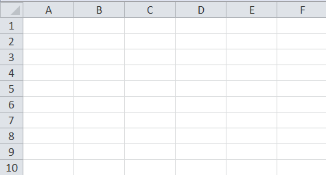
In this example, we will see how to add and remove Excel gridlines for the specific sheet. If we open a new workbook, we can notice that all the sheets will contain grid lines which are shown below.
We can see that the entire sheet contains light grey lines, which separate this as rows and columns. We can edit and add thick borders to these gridlines, or we can remove the gridlines by disabling the gridlines option by following the below steps.
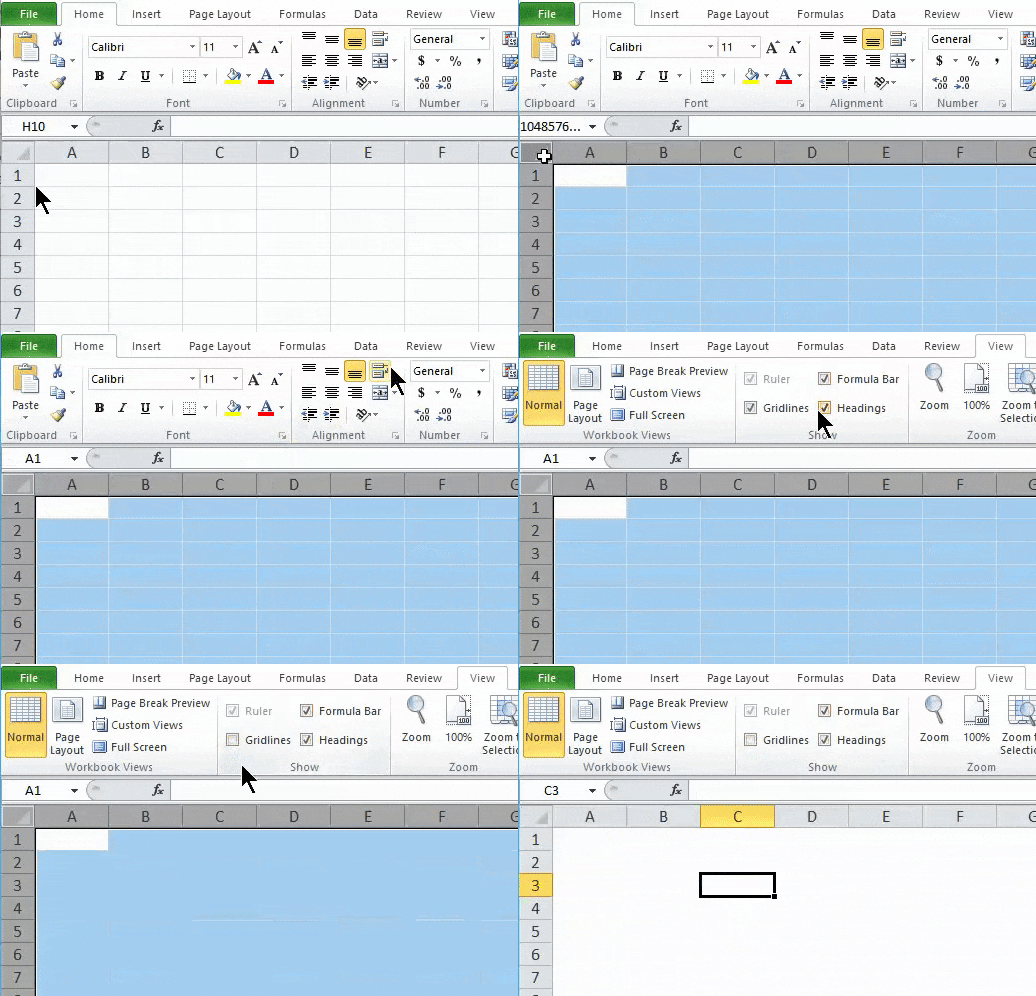
- First, select the entire blank sheet. Go to the view menu, where we can find the gridlines option. We can see that the checkmark has been enabled for the gridlines option. Remove the checkmark for the gridlines so that the entire sheet gridlines will be removed.
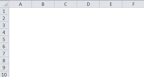
Result:
In the below screenshot, we can see that gridlines have been removed, and it shows plain white paper where we can take a printout without grid lines. Similarly, we can bring back the grid lines for the sheet by enabling the gridlines option in the View menu or the page layout menu.
Example #2
Adding Gridline to the specific sheet
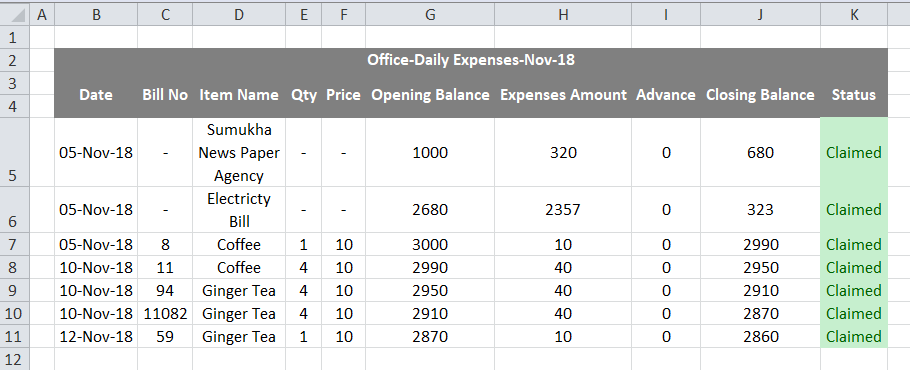
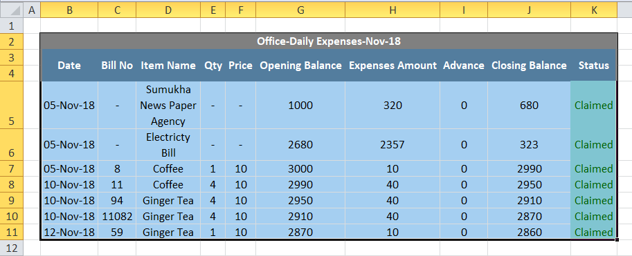
Let’s consider the below example, which shows the expenses data, which contains rows and columns as shown below.
In the above screenshot, we can see that grid lines separate the expenses sheet by rows and columns; we can add or remove the grid lines by following the below steps.
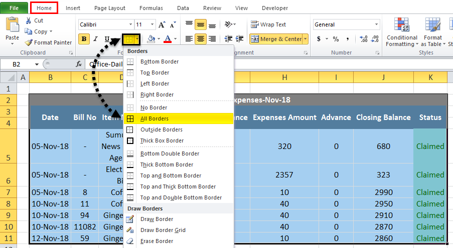
- First, select the data.
- Go to the home menu and add a border to the gridline, as shown below.
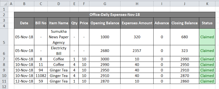
- Once we click on the borders, the selected data will be filled with borders, as shown below.
We can see that expenses data has been filled with borders that give a good view, but the outer sheet contains gridlines; we can hide the outer part of the grid lines by following the below steps.
- First, select the entire sheet as shown below.
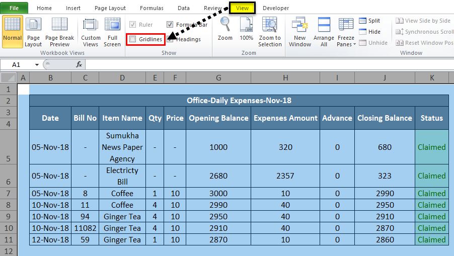
- Go to the View menu, where we can find the gridlines option. Remove the checkmark for the grid line option as shown below.
- In the above screenshot, we can see that the gridlines option has been disabled, which removes the grid line for the full sheet of the outer part, which is shown as the screenshot in the below result.
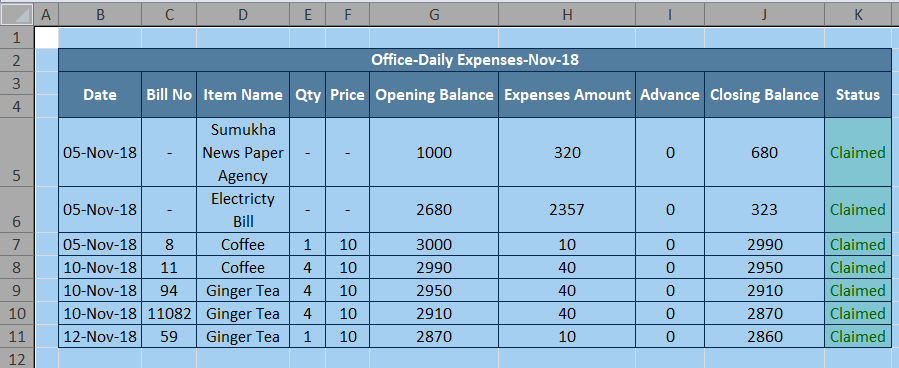
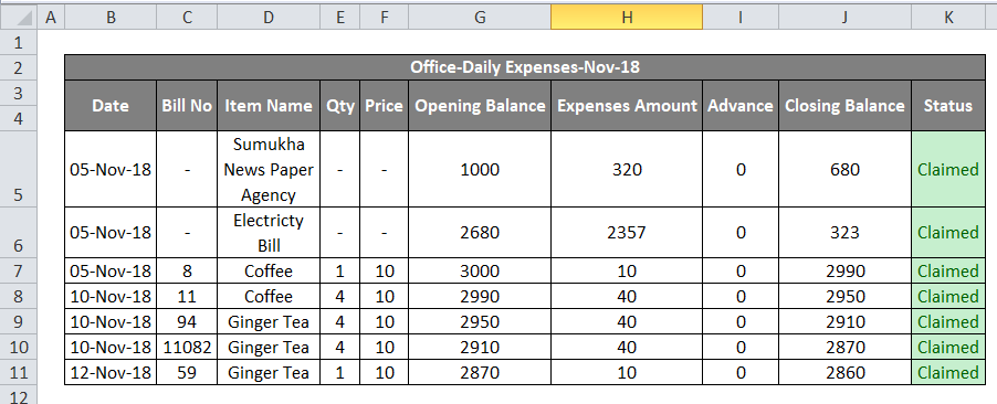
Result:
In the below screenshot, we can see that the outer part of the sheet has no grid lines, and only the specific row and column has the grid lines border. This kind of view will make the sheet to view the data in a professional way.
Example #3
Adding Color to the Excel Gridlines
In this example, we will see how to add color to the grid lines by following the below steps.
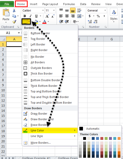
- First, open a new workbook. We will get a sheet with gridlines in a light grey color. Go to the Home menu, where we can find the Border under the font group and get the list of border styles shown below. Choose a line color from the border list.
- Once we click on the line color, we will get the standard and theme color for color selection, as shown below.
- Choose a specific line color; for example, we will choose green.
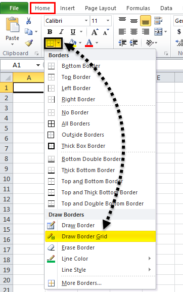
- Go to the same border option and click “Draw Border Grid”, which is shown below.
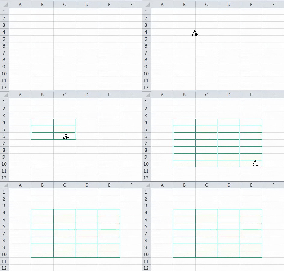
- Now draw the border grid in the specific area where we will get the grid border in the selected green color.
Result:
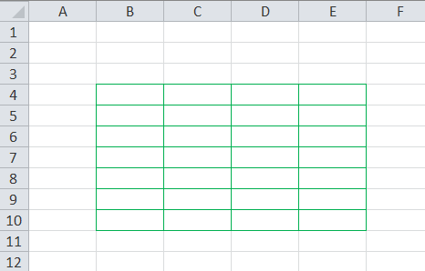
The screenshot below shows that the grid line has been filled with green for the specific rows and columns.
Example #4
Print Gridlines in Excel
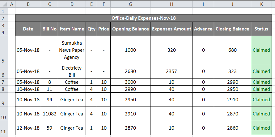
In this example, we will see how to add and remove grind lines while printing the data. Consider the below example, which shows expenses data which is shown below.
Now we can add or remove print gridlines by following the below steps.
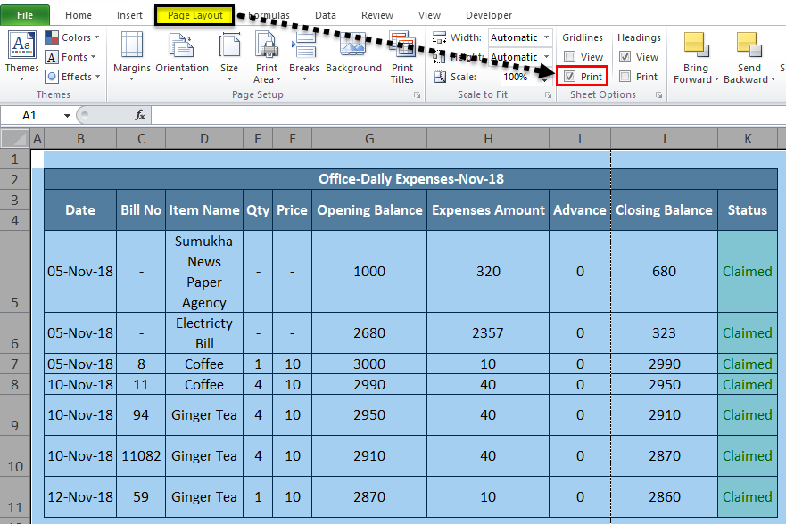
- First, select the entire worksheet. Go to page layout. In page layout where we can see the grid lines under the “Sheet Option” Group
- Enable the Gridlines by check-marking the print option shown in the screenshot below.
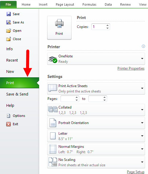
- Use CTRL+P or go to the File menu and give a print. Once we give print, we will get the below print options dialog box which is shown below.
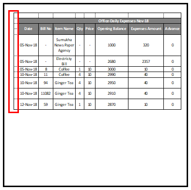
In the print option, we can see the preview on the right-hand side, where we can see the gridlines with light dotted lines which are highlighted below.
- Hit the print button to get the print with grid lines, and in the same way, we can hide the print gridlines by disabling it or removing the tick mark from the checkbox.
Things to Remember About Gridlines in Excel
- In Excel, we can easily remove the gridlines by removing the checkbox in the view menu.
- You can add or remove gridlines in Excel using the keyboard shortcut ALT+W+V+G.
Recommended Articles
This has been a guide to Gridlines in Excel. Here we discuss how to add and remove Excel gridlines, practical examples, and a downloadable Excel template. You may also look at these suggested articles to learn more –


