Excel Header and Footer

Updated August 11, 2023

Header and Footer in Excel

Header and footer in excel are part of page settings that are use to make any worksheet or workbook better for printing. We can add Page Number, Heading, Topic and Chapter name, Company name, Logo, Author’s name and version of a publication, etc. To apply Headers and Footers in Excel, go to the Insert menu tab under the Text section; we have the option Headers and Footers. Once we type any text, it will be marked on all the pages. Go to Footer and from the Design menu tab to insert the page numbers and select the Page Number option. There we have different types of formats to apply for a single thing.

How to Add Header and Footer in Excel?

To add a Header and Footer in Excel is very simple and easy. Let’s understand how to add a Header and Footer in Excel with some examples.

Example #1

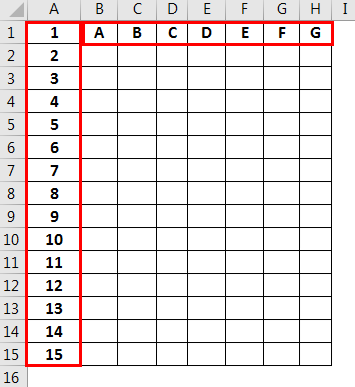
First, fix the top and first columns of the Excel sheet by marking the first column with 1-15 numbers and the top row with A-G Alphabets. (You can use any indices as per your need), Doing this will fix the page length to see the final page layout.

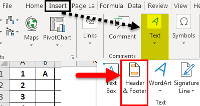
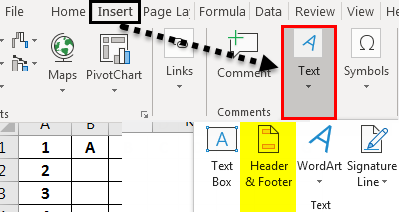
To add a Header and Footer in the Excel sheet, select the Text option from Insert in the Menu bar and select Header and Footer.

Once you click on Header and Footer option, it will be activated in the currently opened excel sheet.

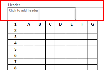
As you can see, the Numbers and Alphabet we entered before have framed the page border to make the page layout. Put the cursor on Click to add header and enter header name as per need.

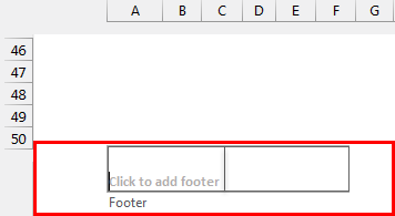
Now go down to enter or change Footer. (If the page size is large, which is normally a default set, go down to change footer)

Put the cursor on Click to add Footer, and enter footer name as per need.

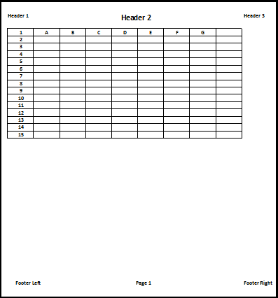
Now to see, how Header and Footer in excel will look like, go to print preview by pressing Ctrl+P or go to Print option in the File menu to see the preview.

Example #2

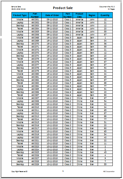
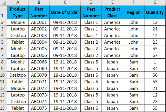
Here we have Product Sale data of a month in this example.

To add Header and Footer in this Excel sheet, go to the Insert Menu bar and select Header and Footer.

Once you click on Header and Footer, the Header and Footer option will be activated in the current opened Excel sheet. Here, our data is arranged in a page set with all table columns on a single page.

Now click on the Header tab, and it will be to be filled with text.

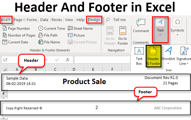
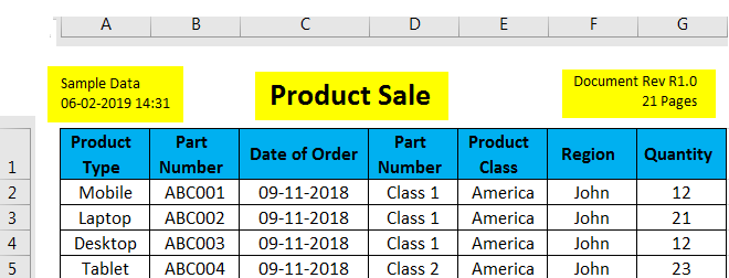
Now you can customize the header by formatting table names, revision numbers, and data types with different fonts and sizes. Below, we can see the main Product Sale in the main header, which is in bold and high in text size; the document revision number and Document type as Sample Data are kept in the corner of the Header.

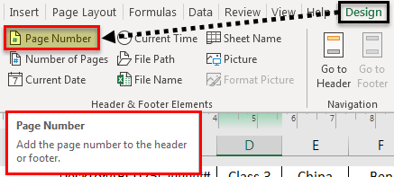
Now, here we will see another step of adding page numbers. For that, go to any page or footer of the first page and click the Page Number tab from the Design option in the Header and Footer Tools menu. This will enable the cell where you want to see Page Numbers in every sheet.

Once you click on the Page Number tab, the selected will be added with “&[Page],” which is nothing but the starting page number “1”. This will be visible when you change the cell or come out from edit mode from the same cell.

By escaping edit mode from that footer, page numbers will start forming sequentially, which will be created in all the subsequent pages as below.

Also, in Footer, you can enter the Copyright detail or number, and your company’s name, if the format allows you to do so. Below, we have filled the footer with some data.

As you can see in the above screenshot, we have put the company’s name, ABC Corporation, in a light color to make a watermark impression and kept CopyRight Reserved © in small fonts. You can use your format as well.

There are additional functions in Excel to enhance the appearance and professionalism of Header and Footer sections.

We have seen how Header, Footer, and Page Number work. Now we will see a few more functions, as shown in the below screenshot.

• Number of Pages – It shows the total number of pages where complete data are available. (Formula = &[Pages])
• Current Date – It gives the current or today’s date. (Formula = &[Date])
• Current Time – It gives the current or publishing time. (Formula = &[Time])
• Sheet Name – It gives the sheet’s name, entered in a sheet to be shown in the Header or Footer. 
• (Formula = &[Tab])
• File Name – Same as Sheet Name, It also gives the name of the file to be shown in the Header or Footer (Formula = &[File])
• Go to Header/Go to Footer – These are used as a shortcut path to go in Header and Footer directly, instead of using a scroll bar to do up and down.

The design menu bar has one Option; we can change the page setting, Margins, Alignments, and Scaling of the document per its own defined standards.

After entering complete data and using all functions available in Excel, we’ll be having our Header and Footer page setup as below;

Pros of Header and Footer in Excel

If you want to present the data in printable form, then Header and Footer in excel make the layout attractive.

• Adding Header and Footer in Excel saves time by automatically adding Heading, Page Number, Revisions, Copy Right to all sheets. No need to add them one by one.
• It saves time to change the Header and Footer of each sheet by doing it manually.

Things to Remember

• Apply header and footer names to all sheets to avoid making changes individually for each sheet.
• If a table has no cell borders, it will appear crowded in the print preview without any visible borders.

Recommended Articles

This has been a guide to the header and footer in Excel. Here we discuss how to add a header and footer in Excel and print a preview, practical examples, and a downloadable Excel template. You can also go through our other suggested articles –

1. Column Header in Excel
2. Excel Header Row
3. Excel Rows and Columns
4. Freeze Columns in Excel