Updated June 2, 2023
Excel Hide Formulas (Table of Contents)
Introduction to Hide Formula in Excel
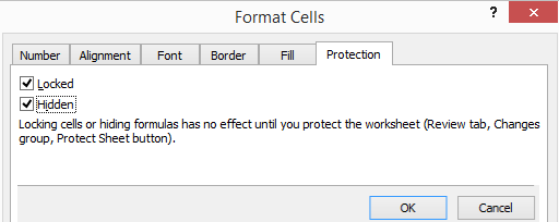
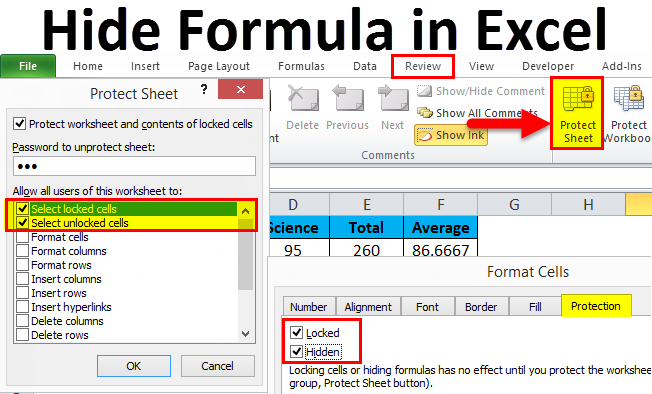
There are two ways to Hide any formulas in Excel. The first way we can protect the current worksheet or workbook is from the Protect Sheet and Protect Workbook option, which is available in the Review menu under the Changes section. There we need to provide the password to lock the changes in Sheet. This will prevent other people from changing their formulas. And other is by Format Cells option, which can be accessed by short cut key Ctrl + 1. From the Format Cells box, under the Protection tab, select the Hidden option and locked option. By doing this, it will lock the selected cell preventing it from editing.
- This feature in Excel is introduced to hide the formulas from others.
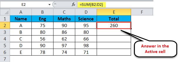
- When writing a formula in an active cell, Excel automatically displays the formula in the formula bar.
- Sometimes, it is necessary to hide the formula for security or confidentiality reasons. In that case, we use the Excel hide formula.
- Excel makes it simple to hide formulas from getting changed.
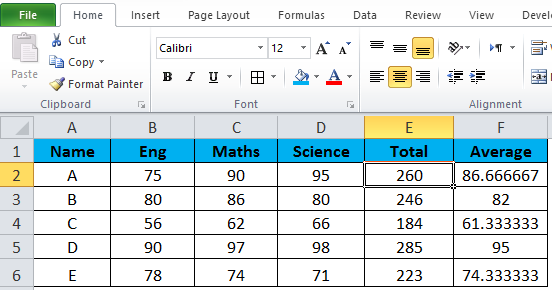
Example:
Different Ways to Hide the Formula in Excel
There are different ways of hiding Excel formulas to protect against accidental or intentional changes in the worksheet, as mentioned below –
- To protect the worksheet and activate the hide formula option.
- To hide the formula bar of the workbook.
#1 – To protect the worksheet and activate the hide formula option.
Steps to hide the Excel formula
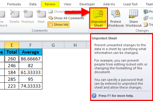
Step 1: To Unprotect the Sheet
- The first step is to make sure that the worksheet is unprotected.
- Go to the Review tab in the Excel ribbon to check the same.
- If you find the Protect Sheet button in the toolbar, then it means the worksheet is not protected. In that case, you can directly start the steps to hide the formula.
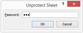
- If you find the Unprotect Sheet button in the toolbar, then it means the worksheet is protected. Click on the same and unprotect the sheet by typing the correct password.
Step 2: To hide the Formula in Excel.
- As per the in-built feature of MS Excel, by default, the active cell formula appears in the formula bar.
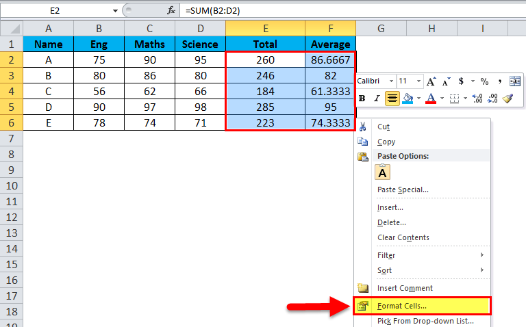
- To hide the Excel formula, you need to select the range of cells for which you want to hide the formula.
- Right-click the cell or range of cells. Select Format Cells or press Ctrl+1.
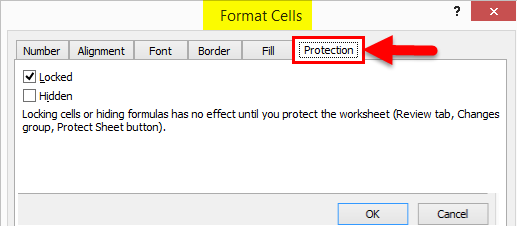
- Once the Format Cells dialog box appears, click on Protection.
- By default, Excel selects the “Locked” checkbox and deselects the “Hidden” checkbox. The selected Locked check box prevents the user from changing the contents of the cells in a sheet, whereas the Hidden checkbox is an optional feature. It helps hide the formula and prevents the user from seeing the same. It needs to select manually.
Step 3: To Protect the Sheet
- This step is very important in hiding the formula. The above formula will remain ineffective until the sheet is protected.
- Go to the Review tab in the Excel ribbon. Click on Protect Sheet.
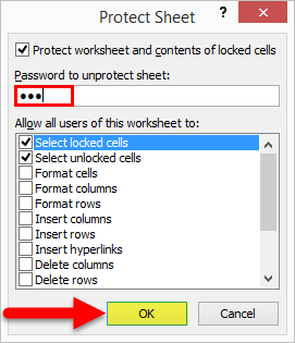
- Protect Sheet dialog box will appear. Type the password to protect the sheet. Once the sheet is protected, no one except the real user can unprotect it, make changes, and then click OK.
Note: By default, Protect worksheet and contents of the locked cells check box are selected. Also, Select locked and unlocked cell checkboxes to remain selected by default.
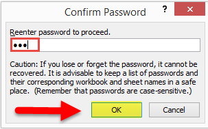
- Retype the password, which will help to prevent a typographical error in the password from locking the spreadsheet forever. Confirm Password dialog box will appear. Click OK.
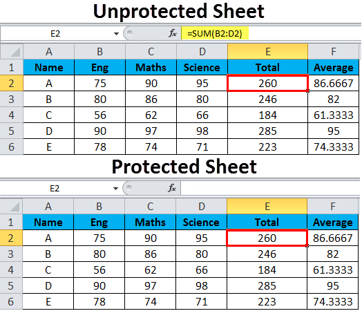
- Once you protect the sheet, the formula of the active cell will not be shown up in the formula bar. Thus, the formulas in the cells are protected and cannot be seen or edited.
- Whenever you want to make changes to the protected sheet, the following message will be displayed.
Note: The user without a password can click on the cells but cannot make changes to the content of the protected sheet. To make the changes, first, make the protected sheet unprotected.
How to Unprotect the Protected Sheet?
- Select the Review tab in the Excel ribbon. Click on Unprotect Sheet option.
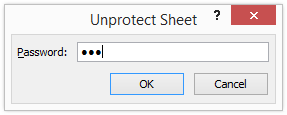
- Unprotect sheet dialog box will appear. Type in the password and then click Ok. The sheet will become unprotected.
#2 – To hide the formula bar of an Excel workbook
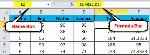
The formula bar exists below the formatting toolbar or ribbon area. It is divided into two different parts:-
The left part is the Name box displaying the active cell number.
On the right, Excel displays the formula of the active cell.
Steps to hide the formula bar:
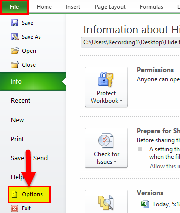
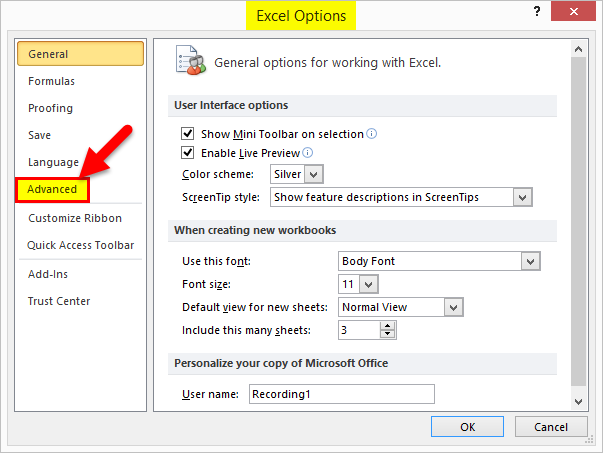
- Go to the File tab in the Excel ribbon. Select Options.
- The Excel Options dialog box will appear. Select Advanced.
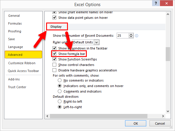
- On the right-hand side panel, scroll down to the Display section.
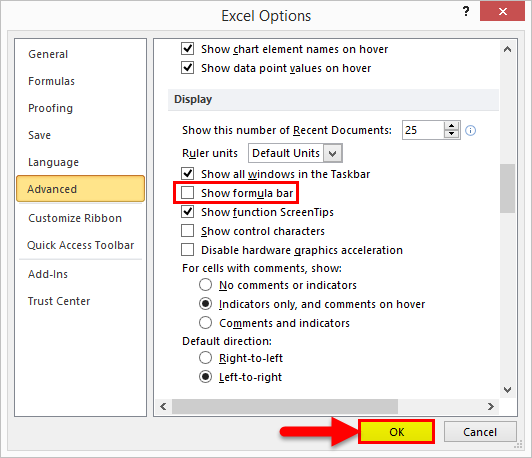
- Unselect the Show formula bar checkbox and then click OK.
Note: If you select the “Show formula bar” checkbox, Excel will display the formula bar; otherwise, it will not be displayed.
How can the Hidden formulas be found?
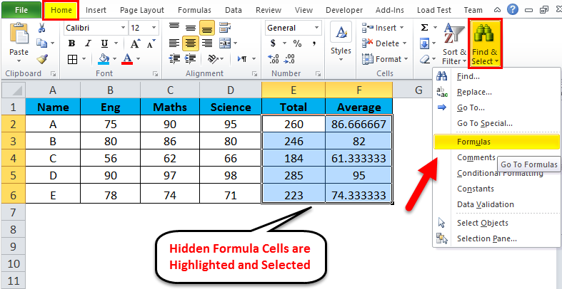
- Go to the Home tab in the Excel ribbon in the Editing section, select Find & Select, and then click the Formulas option.
- Excel will highlight and select all the cells that have formulas.
Things to Remember about the Hide Formula in Excel
- This option helps you hide crucial and confidential formulas from others, thus protecting your documents.
- As discussed above, there are two ways of hiding formulas. In the first method, we can hide and protect the formulas sheet-wise. In other words, in the same workbook, we can apply it to protect and hide the Excel formula in one sheet, whereas the second sheet remains unprotected.
- In the protected worksheet, we can only see the data and put the cursor on the cells but cannot view the formulas and make changes to them.
- The second way to hide the formula bar applies across any file opened in the MS Excel application. However, formulas remain hidden because of the aforementioned feature. The worksheets are not protected.
Recommended Articles
This has been a guide to Hiding Formula in Excel. Here we discuss how to use Hide Formula in Excel, practical examples, and a downloadable Excel template. You can also go through our other suggested articles-

