Updated June 8, 2023

Overview of Hierarchical Clustering Analysis
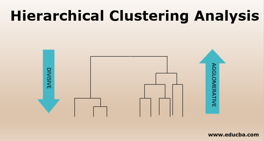
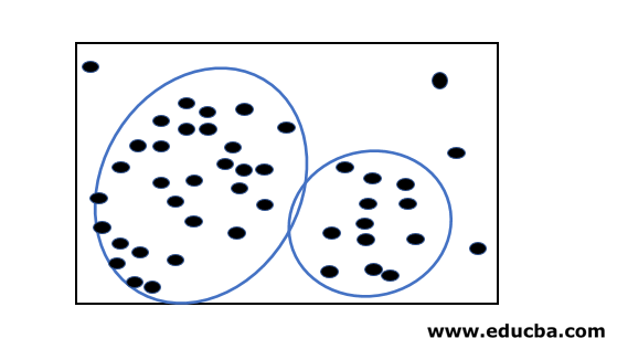
Hierarchical Clustering analysis is an algorithm to group data points with similar properties. These groups are termed clusters. As a result of hierarchical clustering, we get a set of clusters where these clusters are different from each other. Clustering of this data into clusters are classified as Agglomerative Clustering( involving decomposition of cluster using bottom-up strategy ) and Divisive Clustering ( involving decomposition of cluster using top-down strategy )
There are various types of clustering analysis; one such type is Hierarchical clustering.
Hierarchical clustering will help in creating clusters in a proper order/hierarchy. For example, the most common everyday example is how we order our files and folders in our computer by appropriate hierarchy.
Types of Hierarchical Clustering
Hierarchical clustering is further classified into two types, i.e., Agglomerative clustering and Divisive Clustering (DIANA)
Agglomerative clustering
In this case of clustering, the hierarchical decomposition uses a bottom-up strategy, which begins by creating atomic (small) clusters by adding one data object at a time. The atomic clusters are merged iteratively until a large cluster is formed at the end, which satisfies all the termination conditions. This procedure is iterative until all the data points are brought under one big cluster.
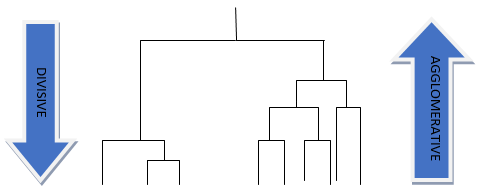
AGNES (AGglomerative NESting) is an agglomerative clustering combining data objects into a cluster based on similarity. The result of this algorithm is a tree-based structure called Dendrogram. Here it uses the distance metrics to decide which data points should be combined with which cluster. It constructs a distance matrix, checks for the pair of clusters with the smallest distance, and combines them.
The above figure shows Agglomerative vs. Divisive clustering.
Based on how the distance between each cluster is measured, we can have 3 different methods.
- Single linkage: The method defines the distance between clusters as the shortest distance between two points within each cluster.
- Complete linkage: In this case, we will consider the longest distance between each cluster’s points as the distance between the clusters.
- Average linkage: Here, we will take the average between each point in one cluster to every other point in the other cluster.
Now let’s discuss the strengths & weaknesses of AGNES; this algorithm has a time complexity of at least O(n2); hence it doesn’t do well in scaling, and one other major drawback is that whatever has been done can never be undone, i.e., If we incorrectly group any cluster in an earlier stage of the algorithm then we will not be able to change the outcome/modify it. But this algorithm has a bright side. Since many smaller clusters are formed, it can be helpful in the discovery process. It produces an ordering of objects that is very helpful in visualization.
Divisive Clustering (DIANA)
Diana stands for Divisive Analysis; this type of hierarchical clustering works on the principle of a top-down approach (inverse of AGNES) where the algorithm begins by forming a big cluster. It recursively divides the most dissimilar cluster into two and continues until all the similar data points belong in their respective clusters. These divisive algorithms produce more accurate hierarchies than the agglomerative approach but are computationally expensive.
The above figure shows the Divisive clustering step-by-step process.
Multiphase Hierarchical Clustering
To improve the quality of clusters generated by the above-mentioned hierarchical clustering techniques, we integrate our hierarchical clustering techniques with other clustering techniques called multiphase clustering. The different types of multiphase clustering are as follows:
- BIRCH (Balanced Iterative Reducing and Clustering using Hierarchies)
- ROCK (RObust clustering using links)
- CHAMELEON
1. Balanced Iterative Reducing and Clustering using Hierarchies
This method primarily employs hierarchical/micro clustering in the initial phase and macro clustering/iterative partitioning in the later phase to cluster large amounts of numeric data. This method overcomes the scalability problem faced in AGNES and enables the ability to undo the actions performed in the previous step. BIRCH uses two critical concepts in its algorithm
a. Clustering feature (Helps in summarizing the cluster)
CF is defined as <n, LS, SS> (n- number of data points in the cluster, the linear sum of n points, the square sum of n points). Storing the feature of a cluster helps avoid storing detailed information about it, and CF is additive in nature for different clusters.
CF1 + CF2 = <n1+n2, LS1+LS2, SS1+SS2>
b. Clustering feature tree (helps in representing a cluster as a hierarchy)
CF tree is a balanced tree with branching factor B (maximum number of children) and threshold T (max number of sub-clusters that can be stored in leaf nodes).
The algorithm works in 2 phases; in phase 1, it scans the database and builds an in-memory CF tree, and in phase 2, it uses the clustering algorithm, which helps in clustering the leaf nodes by removing the outliers (sparse clusters) and groups the cluster with maximum density. The only drawback of this algorithm is that it handles only the numeric data type.
2. Robust clustering using links
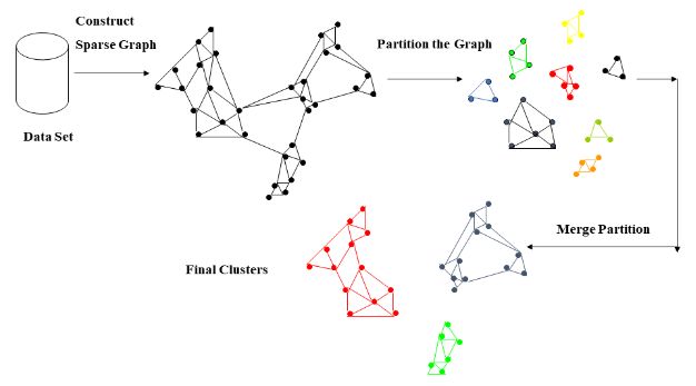
The link between two objects is the number of familiar neighbors they share. ROCK algorithm is a clustering algorithm that uses this concept of linking with the categorical dataset. As we know that the distance-measured clustering algorithms do not provide high-quality clusters for the categorical dataset, but in the case of ROCK, it considers the neighborhoods of the data points as well, i.e., if two data points have the same area, then they are most likely to belong in the same cluster. In the first step, the algorithm will construct a sparse graph considering the similarity matrix with the neighborhood and similarity threshold concept. The second step uses the agglomerative hierarchical clustering technique on the sparse graph.
3. Chameleon
This type of hierarchical clustering algorithm uses the concept of dynamic modeling. It is called dynamic because it can automatically adapt to the internal cluster characteristics by evaluating the cluster similarity, which refers to how well connected the data points are within and near the clusters. Chameleon has the drawback of having a high processing cost, with a worst-case time complexity of O(n^2) for n objects.
Image source – Google
Conclusion
This article has learned what a cluster is and what cluster analysis is, different hierarchical clustering techniques, and their advantages and disadvantages. Each method we discussed has its plus and minus; hence, we need to understand our data with proper exploratory data analysis and choose the algorithm cautiously before going ahead with an algorithm.
Recommended Articles
This is a guide to Hierarchical Clustering Analysis. Here we discuss the overview and different types of Hierarchical Clustering. You may also look at the following articles to learn more –


