Updated March 28, 2023

Introduction to Histogram in Matlab
Histogram is a representation of any statistical information showing the frequency of data items in successive intervals. MATLAB supports plotting histogram feature that enables the user to create a bar graph for any vector or matrix and grouping the data into bins using an automatic binning algorithm. For each bin, the area represents the frequency of occurrence of the data, not the height. It supports customization in histogram presentation.
Syntax:
In earlier versions, hist() and histc() were used to generate histogram plots. In later versions those functions are replaced with new functions with advanced capabilities i.e. histogram(), histcounts() and discretize().
The syntax for the above-recommended functions are as follows:
- histogram(X, a1,a2,…..,an)
- histcounts(X, a1,a2,…..,an)
- discretize(X, a1,a2,…..,an)
Where X: Data input in the form of vector or matrix.
a1,a2,…..,an: Attribute values (optional)
Creation of Histogram in Matlab: MATLAB makes it a single click action to create a histogram for any data. A histogram can be created by using the inbuilt function histogram().
Example:
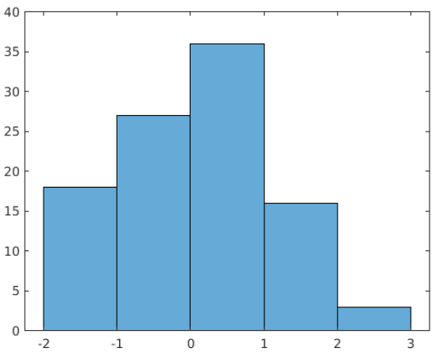
The below code is written to generate 100 random numbers and histogram() is used to plot a histogram for the generated data.
Code:
data = randn(100,1);

h = histogram(data)
Output:
Once any histogram object is created, it can be altered by altering its property values, that makes changes in the properties of bins and thus in the display.
Properties of Histogram in Matlab
Various properties that are featured for the histogram in MATLAB, are as follows:
1. Bins
| Parameter | Description |
| NumBins | Decides the number of bins to be generated. |
| BinWidth | Decides the width of each bin. |
| BinEdges | A vector of which the first element of the vector determines the edge of the first bin and the last element decides the edges of the last bin of the histogram. |
| Binlimits | Sets the limits for the input vector/matrix values. |
| BinLimitModes | Decides mode of setting the limits. |
| BinMethod | Choose the algorithm to configure bin width. |
2. Categories
This property allows to plot histogram for each category defined in the input categorical array. If bin count is specified, categories sets the associated category descriptions in the plot.
This property contains parameters such as mentioned below:
| Parameter | Description |
| DisplayOrder | Decides the order of bars based on height. |
| NumDisplayBins | Decides the number of categories to be displayed. |
| ShowOthers | Decides about the visibility of the additional bar which contains excluded elements of selected categories. |
3. Data
This value gets distributed over a histogram plot among the bins. This property consists of different parameters such as:
| Parameter | Description |
| Values | Decides the number of data elements to be added to a specific bin. |
| Normalization | Applies a specific type of normalization on the data such as count, probability, countdensity, pdf, cumcount, etc. |
| BinCounts | Accepts the bin count as input from an external bin calculation method instead of histogram data binning. |
| BinCountsMode | Represents the mode of deciding bin counts. |
4. Color and Styling
| Parameter | Description |
| DisplayStyle | Decides the style to impose on the histogram display. |
| Orientation | Decides upon the orientation of the bars on the histogram plot- vertical or horizontal. |
| BarWidth | Regulates the separation of categorical bars. |
| FaceColor | Sets the color of the bars. |
| EdgeColor | Sets the color of the edges. |
| FaceAlpha | Decides on the transparency of the bars. |
| EdgeAlpha | Decides on the transparency of the edges. |
| LineStyle | Sets style of the bar outlines. |
| LineWidth | Sets the width of the bar outlines. |
5. Legend
This property in the MATLAB adds descriptive labels to the plots. It comprises of:
| Parameter | Description |
| DisplayName | Sets the text to be added to the description for the axes. |
| Annotation | Controls the inclusion of the objects in a legend and sets excluded objects as an annotation object. |
6. Interactivity
| Parameter | Description |
| Visible | Sets the visibility of an object. |
| DataTipTemplate | Decides on the content that appears on a data tip. |
| UIContextMenu | Sets the context menu for an object, displayed on right-click over the object. |
| Selected | Manages the selection mode of the object. |
| SelectionHighlight | Decides the visibility of selection handlers around an object. |
7. Callbacks
| Parameter | Description |
| ButtonDownFcn | Accepts a function as a value which is to be executed when an object is clicked. |
| CreateFcn | Accepts a function as a value which is to be executed when an object is created. |
| DeleteFcn | Accepts a function as a value which is to be executed when an object is deleted. |
8. Callback Execution Control
| Parameter | Description |
| Interruptible | Determines whether the callback function can be interrupted or not. |
| BusyAction | Determines how the interruption in callback function will be handled. |
| PickableParts | Sets the context menu for an object, displayed on right-click over the object. |
| Selected | Used to enable/disable capturing mouse clicks. |
| HitTest | Decides response on the captured mouse clicks on the Histogram plot. |
| BeingDeleted | Used to store the status of the execution of DeleteFcn callback. |
9. Parent/Child
| Parameter | Description |
| Parent | Axes, Polar axes, Transform objects or Group objects are specified as a parent. |
| Child | This property is a read-only element which is used to view a list of data tips that are plotted in the histogram. |
| HandleVisibility | Accepts a function as a value which is to be executed when an object is deleted. |
10. Identifiers
| Parameter | Description |
| Type | Represents the type of graphic object. |
| Tag | Serves as an object identifier. |
| UserData | Stores arbitrary data on an object. |
Examples of Histogram in Matlab
Let’s understand the usage of different attributes referring to various examples given below:
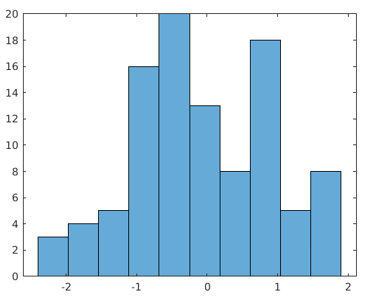
Example #1 – Changing Bin Counts
Code:
data = randn(100,1);

nbins = 10;

h = histogram(data,nbins)
Output:
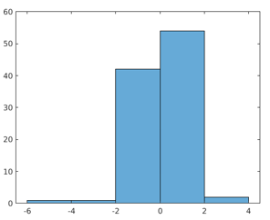
Example #2 – Changing Bin Width
Code:
data = randn(100,1);

histogram(data,'BinWidth',2)
Output:
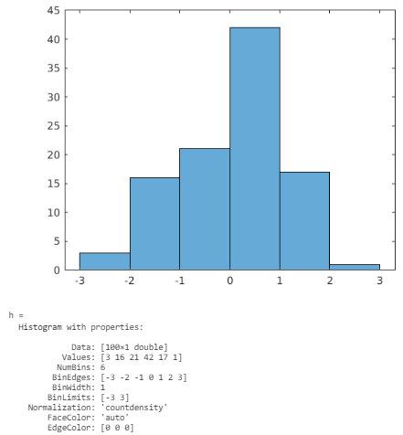
Example #3 – Changing Normalization Type
Code:
data = randn(100,1);

h = histogram(data,'Normalization','countdensity')
Output:
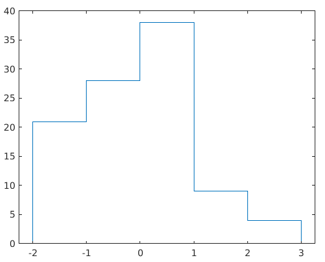
Example #4 – Changing Display Style
Code:
data = randn(100,1);

h = histogram(data,'DisplayStyle','stairs')
Output:
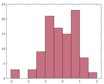
Example #5 – Changing Color of the Bars
Code:
data = randn(100,1);

h = histogram(data,'FaceColor','#A2142F')
Output:
A histogram plot lets you to understand and to analyze the set of continuous data under a frequency distribution. It is advantageous over a bar chart as it allows to divide data into classes in terms of bins which helps to do inspection over a specific category of data as required.
Additional Note:
- The function histogram() creates a histogram object having modifiable properties within.
- Histogram() and histcount() have common built-in options, automatic binning and normalization features.
- The primary calculation function for histogram i.e. histcounts() exhibits consistent behavior.
- Discretize() has extended feature about deciding placements of the bin for each element.
Recommended Articles
This is a guide to Histogram in Matlab. Here we discuss the Creation of Histogram in Matlab and its properties along with its examples and Code Implementation. You can also go through our suggested articles to learn more –
