Updated August 19, 2023
IFERROR in Excel
IFERROR method captures errors in the formula and returns an alternative result or formula when an error is found. We can use the If Error function, where we have even a small chance of getting an error, and we can replace the error message with a customized message we want to see or replace that with a blank.
IFERROR is an easy and structured way to capture and handle errors without resorting to complicated IF statements. Hopefully, by the end of this article, you will know everything you need to know to start using the IFERROR function to improve your Excel skills.
Common Errors in Excel
Below given are some of the errors we can relate to while working in Excel.
It certainly doesn’t look very good, and sadly it’s one of the most common problems people face while writing and using complex formulae in Excel. Whenever Excel encounters something unexpected, which doesn’t sit well with the underlying formula, it returns a value in the form of an error like the ones shown above. Hence, it is always a good idea to cover your expressions or formulae to handle those bothersome corner cases which result in errors. Like every other programming platform, Excel provides an excellent way to handle errors through the IFERROR.
IFERROR falls under the umbrella of Excel’s Logical Functions – as the name suggests, this group of functions uses logical values such as TRUE and FALSE as input or output. To properly understand what IFERROR does, it would help to first look at how the IF function works.
The IF function is one of the simplest logical functions, and it does the following:
- It tests for a condition.
- Based on the outcome of the test above, it performs an action.
- It also provides an alternative course of action in case the condition is not met.
The IFERROR function also works in a similar fashion. But in this case, it tests whether formula or expression would evaluate correctly or whether it would result in an error and returns something depending on the result of this test.
IFERROR Formula in Excel
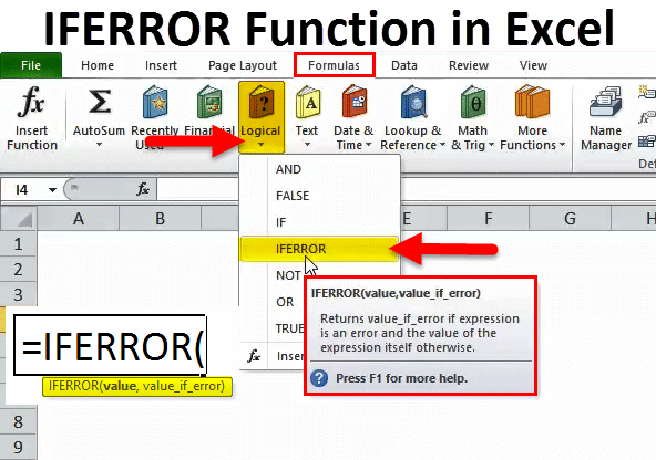
The Formula for the IFERROR Function in Excel is as follows:
So to summarize, the IFERROR Function in Excel would do the following:
- Test an Excel formula or an expression.
- If the expression or formula evaluates an error, it provides you with the option to return a custom value that could be an expression or a formula.
- If the expression or formula doesn’t result in an error, then it will return the result of this formula or expression.
IFERROR can handle any Excel error that one might encounter, including #N/A, #VALUE!, #REF!, and #DIV/0! #NUM! #NAME? and #NULL!
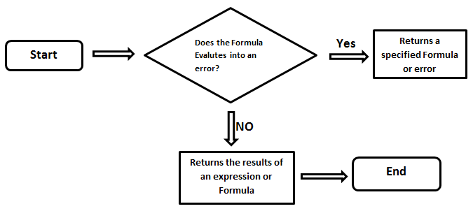
To represent this in the form of a flowchart, it would look like this:
The basic objective here is to catch the errors, handle them effectively, and thereby elevate the overall user experience – and that is the main goal.
How to Use IFERROR Function in Excel?
IFERROR Function in Excel is very simple and easy to use. Let us understand the working of IFERROR in Excel with Some Examples.
Example #1 – Handling #N/A Error
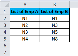
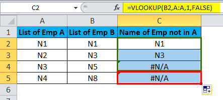
Suppose we have two lists of employees in Columns A and B. In Column B, there are some employees which are not there in Column A. We want to find out the names of those employees who are not in Column A.
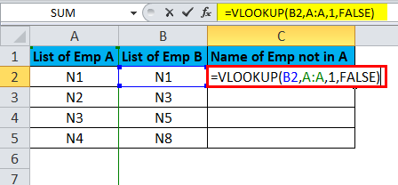
So we will apply the VLOOKUP formula to the right of Column B. The formula for VLOOKUP is shown below.
We shall write the formula for cell C2.
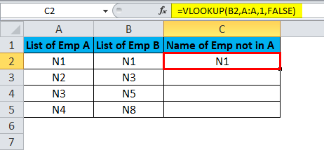
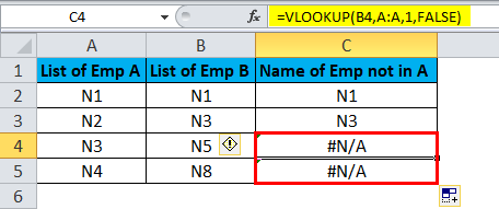
And then, left-click, hold, and drag the mouse to drag the formula down the rest of the list.
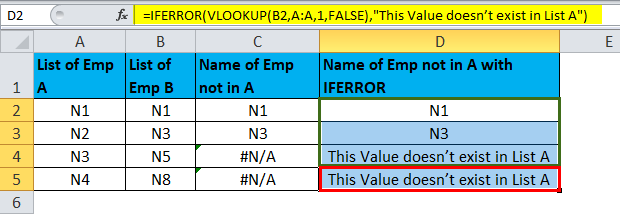
As we can see, there are some names that could not be found in Column A. Hence VLOOKUP generated a #N/A error for those rows.
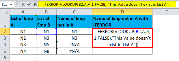
If we want #N/A to be replaced by some other value, such as “This Value doesn’t exist in List A”, then we shall use the IFERROR function.
So we will pass the VLOOKUP formula as the first argument in the IFERROR function – in value.
Next, we will pass “This Value doesn’t exist in List A” as the value_if_error.
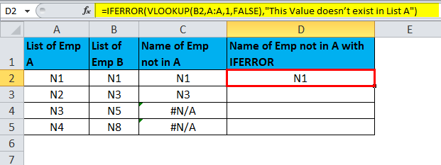
The result is:
After this, we will left-click and hold the mouse to drag the formula to the entire column. This will copy the formula to the rest of the rows and gives the results.
Example #2 – Handling #NULL! Error
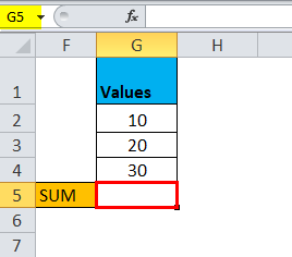
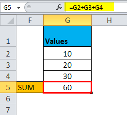
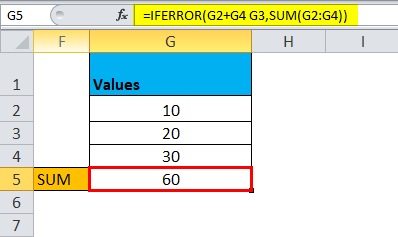
Suppose we have 3 values in cells G2, G3, and G4. Our objective is to sum them in cell G5.
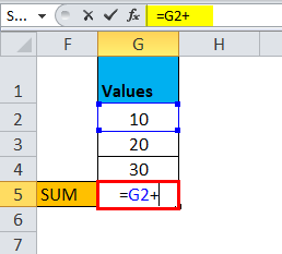
So we start writing the formula using the ‘+’ operator to add the numbers.
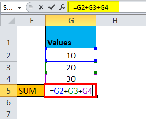
Normally we do this like this:
And this yields the following result:
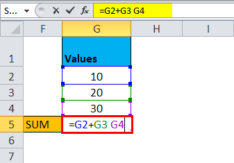
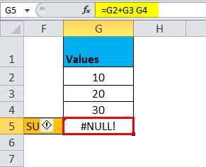
Now suppose, instead of ‘+’, we entered a space or pressed any other incorrect key in this formula.
It will result in an error.
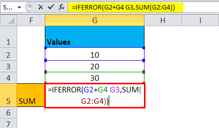
So to rectify this error, we can use the IFERROR function by passing the summation formula in the first argument – value.
Next, we will pass the correct formula in the value_if_error argument.
This is correct the above error and gives the right result.
It will return the result:
Example #3 – #DIV/O!
Let us imagine a scenario to understand this better. Suppose you are a Director of a large gift store chain with outlets nationwide. You receive a monthly report showing some basic figures related to overall sales achieved in all different states, split among 5 sales managers the company employs. Your job is to check this report and then forward it to your colleagues on the Board so you can together analyze the data and formulate a plan to counter dips or capture further opportunities.
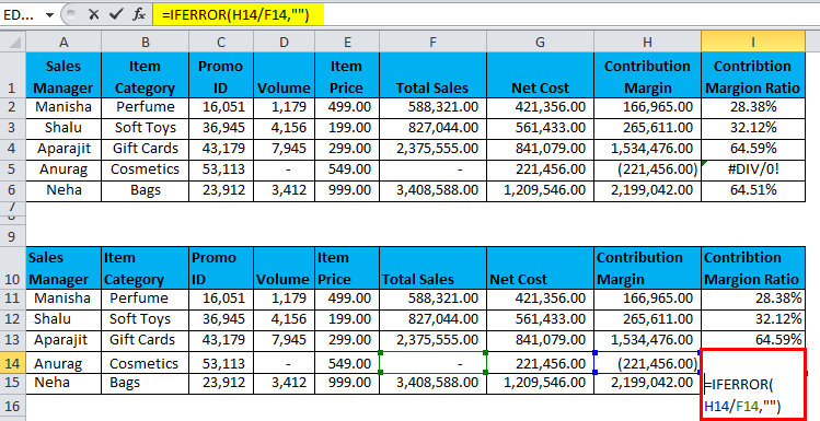
If on opening one such report, you see something like this:
Does it look good to send this report as it is to the rest of the Board?
I wouldn’t. The #DIV/0! sticks out like a sore thumb, and for high stake meetings, having these visual sores in your Excel report is a downright embarrassment. So how does one clean this? This is where the IFERROR Function comes to your rescue. The IFERROR function allows you to replace all such errors as shown above with a suitable value, expression, or function of your choice. In the scenario described above, you can leave the cell black using IFERROR Formula.
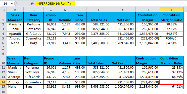
The IFERROR Function returns the result as:
In the scenario described above, we use the IFERROR function to handle a #DIV/0! Error. This error is caused when either:
- dividing by 0 or
- dividing by a cell that has no value.
The last column of this table, ‘Contribution Margin Ratio’, divides the Contribution Margin of a sales manager by its Total Sales. In the case above, Sales Manager Anurag made no sales for that month. Thus, in this case, the Contribution Margin is divided by 0 and the #DIV/0! An error is caused. As shown in the example above, we can use the IFERROR Function to ‘fix’ a #DIV/0! Error. This is one of an Excel user’s most widely encountered situations. Another common situation where most users encounter an error is using the VLOOKUP function, which returns #N/A when it can’t find the value it is searching for. Thus, it is a good idea to use the IFERROR Function in such cases to improve the general look of the report.
Now, it is true that there are other alternatives to this, but IFERROR is perhaps the simplest and the most versatile among them. Let’s discuss why IFERROR is the simplest among all the other alternatives that are available in Excel. If, for some reason, IFERROR is not available for use (and it’s not that unlikely because IFERROR was introduced as late as 2007!).
In that case, we would have to use other formulae to achieve the same result, which is more complicated and quite cumbersome to write.
The Result is:
So which formula looks cleaner and easier to write?
IFERROR not only looks more elegant but also provides a very simple way to handle these situations.
Things to Remember
- Use IFERROR with other functions to cover cases where the functions could return an error. It’s always best to account for these exceptions.
- IFERROR evaluates a function that accepts as an argument and returns an alternative result in error.
- IFERROR replaces the value for all types of errors, i.e. you will get the same custom value for all types of errors.
- If you want to display an alternative value only for #N/A, then consider using the IFNA function instead of IFERROR.
- IFERROR is not available with old versions of Excel (prior to 2007).
Recommended Articles
This has been a guide to IFERROR in Excel. Here we discuss the IFERROR Formula in Excel and how to use IFERROR Function in Excel, along with Excel examples and downloadable Excel templates. You may also look at these useful functions in Excel –


