Updated July 4, 2023
Introduction to INDIRECT Formula
The indirect formula references another cell in Excel. It is a handy formula in Excel which uses a text string as a reference to find a value for that text string. We will see a small example for those who don’t know about referring.
How to Use INDIRECT Formula in Excel?
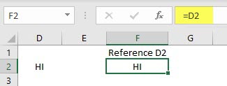
In cell D2, we input a small text, “Hi” Now, in cell F2, we have referred to cell D2; that is the reason in cell F2; also, we have the text “Hi.”
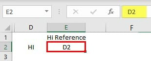
Now we will try differently. In cell D2, we have the text “Hi,” In cell E2 “, D2” is mentioned, which is a reference cell of “Hi.”
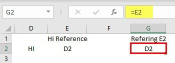
If we call E2 in any cell, it will display only text D2 but not the data in cell D2.
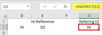
In this kind of situation, the INDIRECT formula will be helpful. For example, when we call E2, it gives the result as D2; if we call E2 with the help of INDIRECT, then it will display the text “Hi.”
That means if we call cell E2 in G2, it will take the data in E2, which is D2, as a reference cell and will call the data in that cell. So, in simple terms, instead of calling the D2 cell directly, we will call the cell with text D2. So, I hope you got a little idea about the INDIRECT formula.
To make you understand the concept, I started with referencing and moved to the INDIRECT function. Now we will see the syntax of INDIRECT, which was not covered earlier. Below is the syntax; it has two parameters one is ref_text, and another is a1.
- Ref_text: The name itself expresses that it is a reference text. If we input a formula like INDIRECT(C2), C2 is the reference text.
- A1: Now, what is a1 here? It is a logical value that will tell about the reference text.
We can refer to using INDIRECT one way if the A1 method means we refer to C4, which implies column ‘C’ row 4 simply we are calling as the a1 method. Another way to represent C4 is R4C3, row 4, column 3. This method is called an R1C1 method.
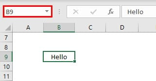
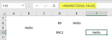
So, if we give TRUE or blank mean, the reference will be considered in the form of the A1 method. A FALSE mean reference will be regarded as the R1C1 method if we provide it. We will see a few examples of these two methods. Now “Hello” is in cell B9.
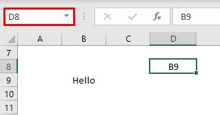
B9 is given as text in cell D8.
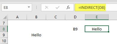
Referring to cell D8 with the INDIRECT formula will give the data in the B9 cell.
A1 method: In this, we can refer to D8 with the INDIRECT method
=INDIRECT(D8)
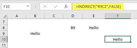
R1C1 method: We can refer to B9 as row 9 and column 2 in this method.
=INDIRECT(“R9C2”, False)
Another way we can refer is if a cell has text R9C2, we can refer to that cell with the INDIRECT formula in the R1C1 method.
In the above screenshot, R9C2 is in cell D10; hence, we refer to D10 in the formula, but the string reference is in the R1C1 method, therefore False.
Examples of INDIRECT Formula in Excel
Below are the different examples of INDIRECT Formula in Excel:
Example #1 – Lock Reference
Using the INDIRECT method, we can lock the reference also. Thus, if we use the reference cell even after adding or deleting the additional row or column, the formula will stay constant with the reference.
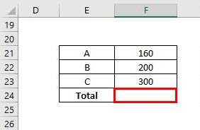
Consider a small table of data as below.
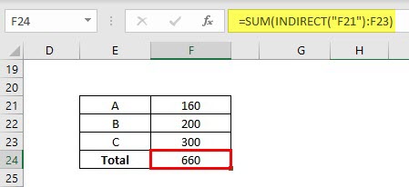
Need to perform SUM calculation by using the INDIRECT function with reference F21.
We need to perform the SUM operation from cell F21 to F23 with the reference as F21; hence keep it in double-quotes closed by brackets as shown in the picture.
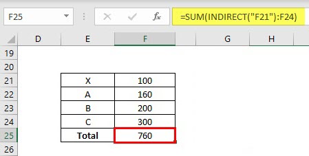
Now we will insert one more line above A and add another value as below picture.
The formula will automatically pick F21 to F24. However, if we perform the same with normal SUM operation, the formula will change from F22 to F24.
Example #2 – Lock Range
We can lock the range and keep the formula standard even when adding or deleting the rows.
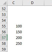
Consider a small range of data from C55 to C58 as below.
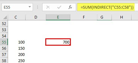
Now we will add the data from C55 to C58 using the INDIRECT formula.
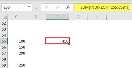
Now we will add one new line between 57 and 58.
Even after entering a new line, the formula remains the same as C55: C58. Therefore, the results of the SUM will change accordingly.
Example #3 – INDIRECT formula using Name Range
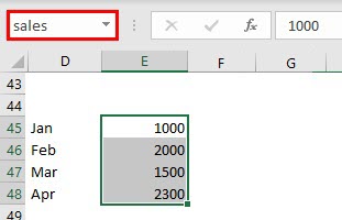
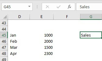
The INDIRECT formula can be applied to the name range also. But first, give a name to a range of numbers.
Input the string “sales “in cell G45.
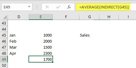
Now find the AVERAGE of sales using the INDIRECT formula.
INDIRECT refers to G45, which has reference string sales; sales is the reference of cells E45 to E48.
Example #4 – INDIRECT Formula with Two Worksheets
Consider the same datasheet. Using the INDIRECT formula, we can dynamically refer to data from different worksheets. Give some name to the sheet-like example below.
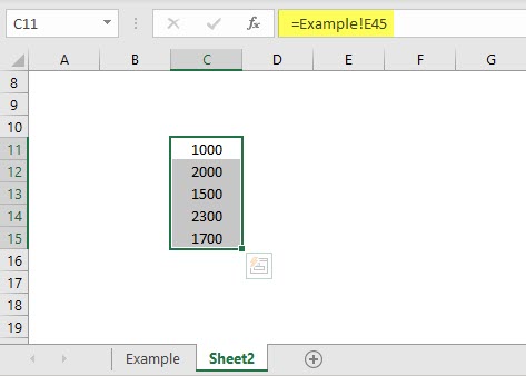
Now we will call the data from the Example sheet to sheet 2. Before using INDIRECT, we will refer in a normal way first.
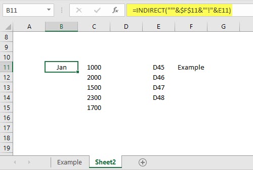
Observe the formula; if we want to refer to other sheet data, the format is “sheet name! cell reference”. But to refer to the INDIRECT function first, we must take the sheet name and cell references in sheet 2. Now apply the INDIRECT function.
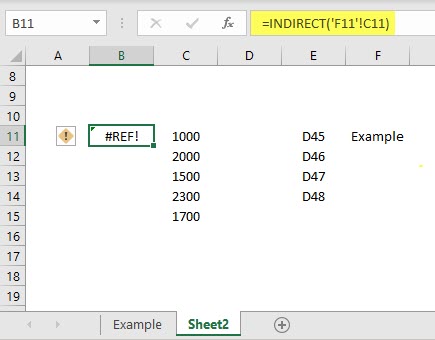
F11 refers to the sheet name, and C11 refers to the Cell reference in the Example sheet. But the formula results in # REF. Because the sheet name should be in string format, keep the cell address in single quotes and then cell reference with concatenation operator.
“ ‘ “ &Sheet name reference &” ’!” &Cell reference
Observe the formula; now, it has given the results from the Example sheet.
Things to Remember
- The indirect formula can be written in two types of A1 method and the R1C1 method. If we do not mention a logical reference, it will automatically consider as the A1 method.
- Lock reference will help to lock a cell or range to make the formula constant.
- While referring to the other sheet, the sheet name should be in string format for using single quotes and concatenation operators.
Recommended Articles
This is a guide to INDIRECT Formula in Excel. Here we discuss How to Use the INDIRECT Formula in Excel, practical examples, and a downloadable Excel template. You may also look at the following articles to learn more –
