Updated August 22, 2023
Excel Inverse Matrix (Table of Contents)
Introduction to Inverse Matrix in Excel
A square matrix for which you want to compute the inverse must be a square one. It means the matrix should have an equal number of rows and columns. The determinant for the matrix should not be zero. If it is zero, you can find the inverse of the matrix. The theoretical formula for computing the inverse of a matrix A is as follows:
Where,
|A| = Determinant of matrix A.
(adj A) = Adjoint of matrix A.
If we put both these values in the formula above, we can get the inverse of any matrix A. It sometimes becomes very tedious to compute a matrix’s inverse. Mathematicians will be happy to know if any function can work for them and compute the inverse of a matrix.
MINVERSE Function to Compute Inverse of a Matrix
Excel MINVERSE function allows a user to compute the inverse of any square matrix with a non-zero determinant. The inversed matrix has the size same as the original matrix. The inverse matrix computed is of the size same as the original matrix.
Syntax:
=MINVERSE(array)
Argument:
Array – Is an array of values representing a matrix.
In this article, we will see how to compute the inverse of a square matrix.
Examples of Inverse Matrix in Excel
Let’s understand how to create the Inverse Matrix in Excel with some examples.
Example #1 – Compute Inverse of a 2X2 Matrix
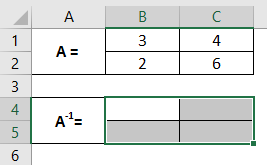
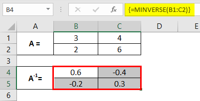
A 2X2 matrix is something that has two rows and two columns. Suppose we have a 2X2 square matrix, as shown in the image below.
Step 1: Decide a range of 4 cells (since we have a 2X2 matrix) in the same Excel sheet, which will hold your inverse of matrix A. Here I have chosen cells A1:C5 as a range for the inverse of matrix A.
These are the ranges where the inverse of matrix A will be computed.
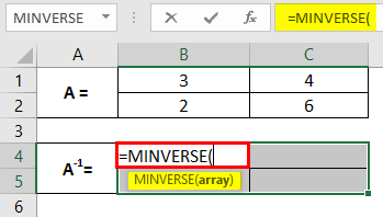
Step 2: In cell B4, start typing the formula for matrix inverse =MINV. You will see the range of formulae associated with the keyword. Double click to select the MINVERSE out of those to compute the inverse of matrix A. Selecting all the cells where your inverse will be computed is mandatory.
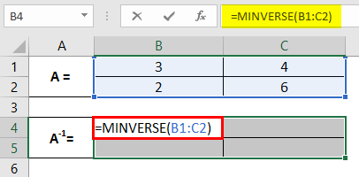
Step 3: Provide an array argument for the MINVERSE function as B1:C2 and close the parentheses to complete the formula. Note that the array we provide as an argument to the function MINVERSE consists of the cells with values for the original matrix A.
Step 4: To see the formula output every time, we must press the Enter key. But in this case, you need to hit Ctrl + Shift + Enter keys so that the formula gets converted into an array formula which looks like this {=MINVERSE(B1:C2)} and works along with all the cells associated with the inverse of A.
You can see across the cells B1:C2 the matrix is inverse of the original matrix A.
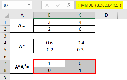
We can also check whether the inverse we get through the MINVERSE function is correctly captured. The way to check it is to multiply matrix A and A-1. The multiplication should result in an identity matrix.
We can achieve matrix multiplication by using the MMULT function in Excel. It multiplies the matrices. See the output in an array of cells B1:C5.
Example #2 – Compute Inverse of a 4X4 Matrix
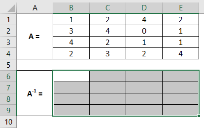
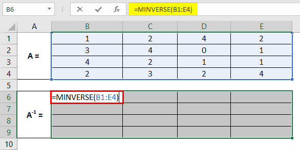
Step 1: Input a 4X4 matrix across the cells A1:E4, as shown in the screenshot below. This is the matrix for which we need to compute the inverse matrix.
Step 2: Select cells from A6 to E9. These are the cells where we will compute the inverse of a 4X4 matrix named A.
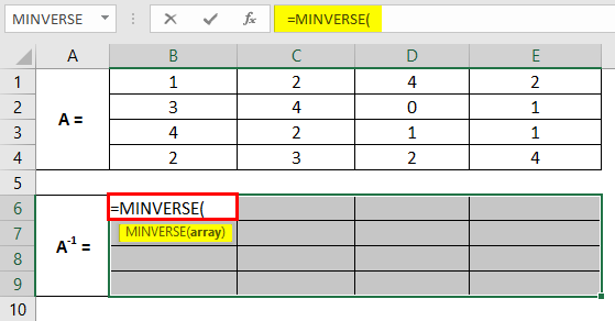
Step 3: Keeping all the cells selected, in cell B6, start typing the formula for matrix inverse as =MINV; through the list of formulae associated with the keyword, double click to select MINVERSE.
Step 4: Use array reference B1:E4 as an array argument to this function and close the parentheses to complete the formula.
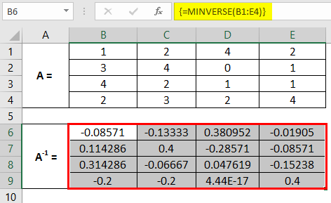
Step 5: Instead of pressing the Enter key, press Ctrl + Shift + Enter keys simultaneously to compute the inverse values for all the cells across B1:E4. If you do not do this, the formula will not be converted into an array formula and will be applied only to the current cell, and if you try to drag it for other cells, it will give you an error.
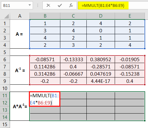
This is how we can compute the inverse of a matrix in Excel using the MINVERSE function. We can also check with the help of the MMLUT function whether the inverse is computed rightly or not.
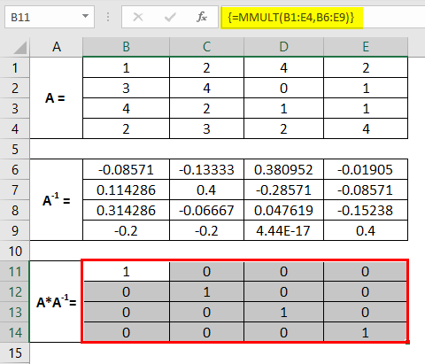
Select the ranges from B1 to E9, where we can check whether the multiplication of these two matrices is an identity matrix.
It comes as an identity matrix. Therefore we can say that the inverse we captured is rightly captured. This is it from this article. Let’s wrap things up with some points to be remembered.
Things to Remember
- If there is any blank cell or non-numeric value in a given matrix, MINVERSE will give you #VALUE! Error.
- If you select some extra cells in the resulting matrix, you will receive a #N/A error.
- If a given matrix is a singular matrix (for which the inverse does not exist), you will receive #NUM! Error.
- It is recommended to use MINVERSE as an array formula. Otherwise, you may get some weird results across the cells. Like getting value errors when you drag and drop the formula across the rows.
- If you don’t want to use it as an array formula, you must input the same formula across all the cells to get the result.
Recommended Articles
This is a guide to Inverse Matrix in Excel. Here we discuss How to create Inverse Matrix in Excel, practical examples, and a downloadable Excel template. You can also go through our other suggested articles –
