Updated May 3, 2023
IPMT Function in Excel
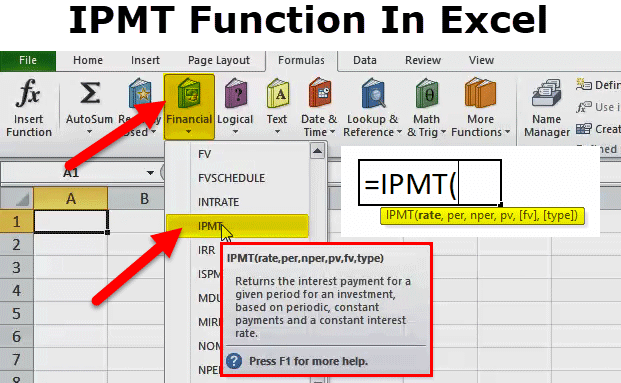
IPMT Function calculates a specific portion of interest based on the loan amount and tenure. The syntax of IPMT is quite similar to the syntax of PV Function in Excel, which all have seen earlier. To understand better, IPMT helps used to distinguish between different portions or segments of any loan and to what time how small amount is to be paid based on the interest applicable can be calculated.
IPMT Formula in Excel:
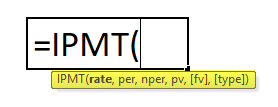
Below is the IPMT Formula in Excel.
Explanation of IPMT Function in Excel
There are six parameters used for the IPMT function. Four parameters are compulsory, and two are optional.
Parameter details are as follows:
Compulsory Parameters:
- Rate: The interest rate per period.
- Per: The period for which you want to find the interest and must be in the range 1 to n per.
- Nper: The total number of payment periods in an annuity.
- Pv: The present value, or the lump-sum amount that a series of future payments is worth right now.
Optional Parameters:
- [FV]: It is an optional argument. The FV or a cash balance you want to attain after the last payment is made. If FV is omitted, excel assumes it to be 0 (the future value of a loan, for example, is 0).
- [Type]: This is also an optional argument. The number 0 or 1 indicates when payments are due. If this argument is omitted, Excel assumes it to be 0.
The Type can be 0 or 1, where:
0 = The payment is made at the end of the period;
1 = The payment is made at the start of the period.
How to Use the IPMT Function in Excel?
IPMT function in Excel can be used as a worksheet function and a VBA Function. Here are some examples of the IPMT functions to understand the working of the IPMT function in Excel.
Example #1
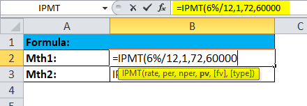
Interest payment made for months 1 and 2 of a loan of $70,000, which is to be paid after 6 years. An interest rate of 6% per year, and the payment to the loan is to be made at the end of each month.
Result is :
- To convert the annual interest rate of 6% into the monthly rate (=6%/12) and the number of periods from years to months (=6*12).
Example #2
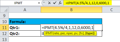
Interest during quarters 1 and 2 of an investment is required to increase investment from $0 to $6,000 over 3 years. The interest rate of 4.5% per year, and the payment into the investment is to be made at the beginning of each quarter.
Result is :
- The annual interest rate has been converted into a quarterly rate (4.5%/4)
- The number of periods has been converted from years to quarters (=3*4).
- The [type]argument has been set to 1 to indicate that the payment will be made at the start of each quarter.
- The interest for the first quarter is zero, as the first payment is made at the start of the quarter.
Note:
* Use N%/12 for rate and N*12 for nper when there are monthly payments. N%/4 for rate and N*4 for nper when quarterly payments and N% for rate and N for nper when there are annual payments.
*Cash paid out is shown as negative numbers. Cash received is shown as positive numbers.
Things to Remember
Below are a few error details that can come in the IPMT function as the wrong argument will be passed in the functions.
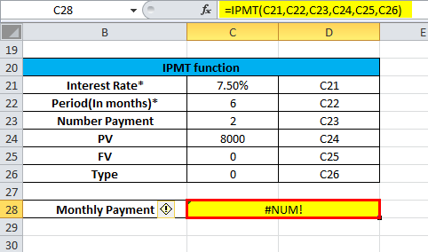
1. Error handling #NUM!: If per value is < 0 or > the value of nper then the IPMT function through a #NUM error.
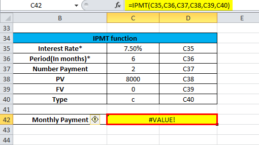
2. Error handling #VALUE!: IPMT function through a #VALUE! Error when any non-numeric.
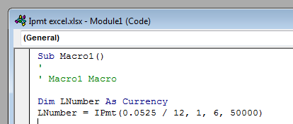
VBA Function Example:
The IPMT function can also be used in VBA code.
For example:
Recommended Articles
This has been a guide to IPMT in Excel. Here we discuss the IPMT Formula in Excel and how to use the IPMT function in Excel, along with practical examples and downloadable Excel templates. You can also go through our other suggested articles –
