Updated August 24, 2023
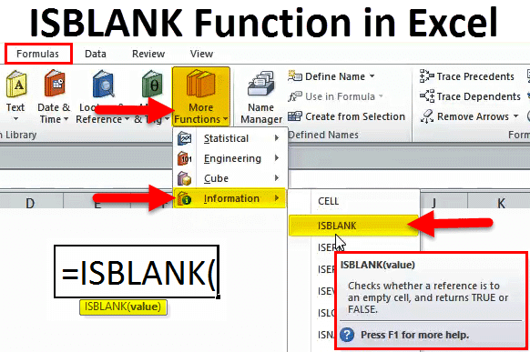
ISBLANK in Excel
The ISBlank function in Excel calculates whether the selected cell is Blank by answering Boolean. If the cell we select is blank, we get TRUE; otherwise, we will get FALSE. It is a simple Boolean function whose answer is a TRUE or FALSE statement that justifies whether the cell is Blank. It is quite useful when we have a huge list of cells, some of which have special characters, or dummy characters will seem just like a blank cell.
ISBLANK Formula in Excel
The Formula for the ISBLANK Function in Excel is as follows:
The Formula of ISBLANK includes only one parameter, i.e. value
Value: This is the targeted cell you want to test.
How to Use ISBLANK Function in Excel?
ISBLANK Function in Excel is very simple and easy to use. Let us understand the working of ISBLANK in Excel by Some Examples.
Example #1
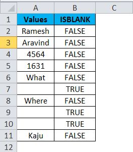
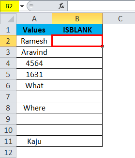
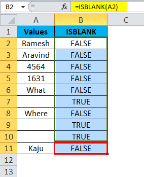
This is the basic example of the ISBLANK Formula in Excel. I have data in column A form A2:A11. I need to check which row has a blank cell, i.e. without any values.
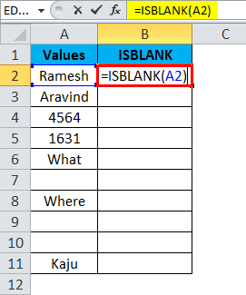
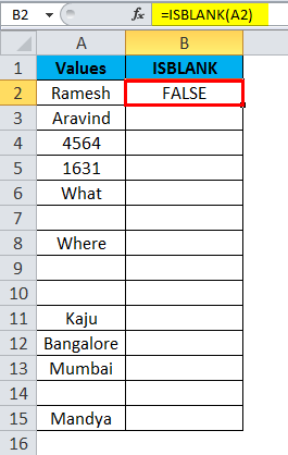
Apply the ISBLANK function in B2
The Formula for ISBLANK Function is given below:
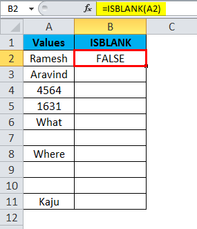
The result is:
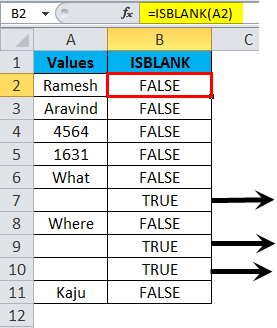
Drag and drop the formula to the remaining cells.
This arrow shows the cell which is blank and returns the value as True.
Example #2
This is an example of a bit advanced. Cleaning the data if our formula shows any errors.
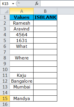
Assume we have data from A2:A15, as shown in the below image.
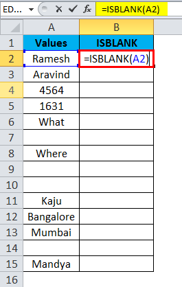
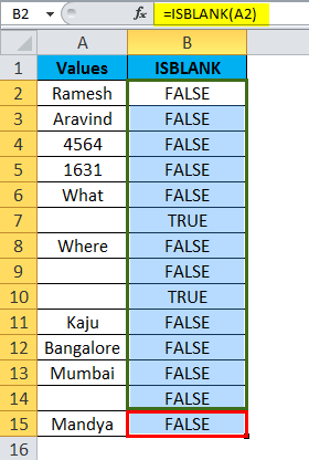
I have applied the formula in column B to check the empty cells.
It returns the result as:
Drag and drop the formula to the remaining cells.
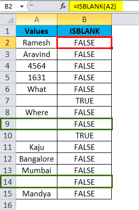
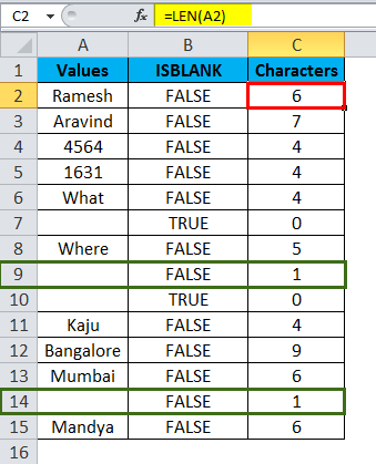
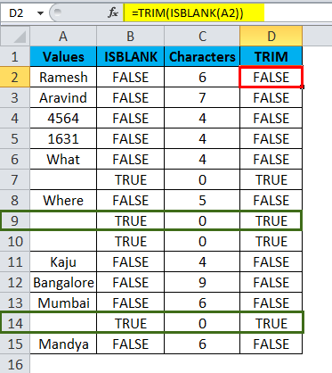
In the above formula, even though the cells A9 and A14 do not have anything, our formula still says there is something in the cells that show the result as FALSE.
Ok, let me clean the data by using LEN and TRIM functions.
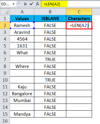
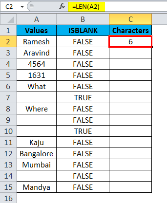
Firstly, I want to check the number of characters in the cell by using the LEN function.
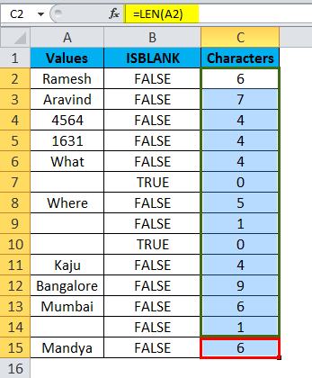
LEN Function returns the result as:
Drag and drop the formula to the remaining cells.
LEN function determines there are characters in the cells.
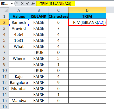
Now I need to clean the cell by using the TRIM function.
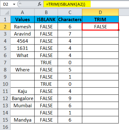
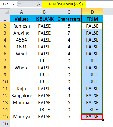
TRIM Function returns the result as:
Drag and drop the formula to the remaining cells.
TRIM function clears all the unwanted spaces and returns the actual values. Since there are no values in cells A9 & A14, now the ISBLLANK formula returns the result as TRUE.
Example #3
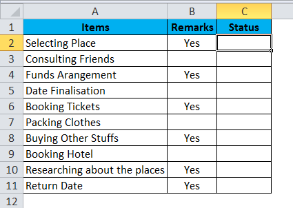
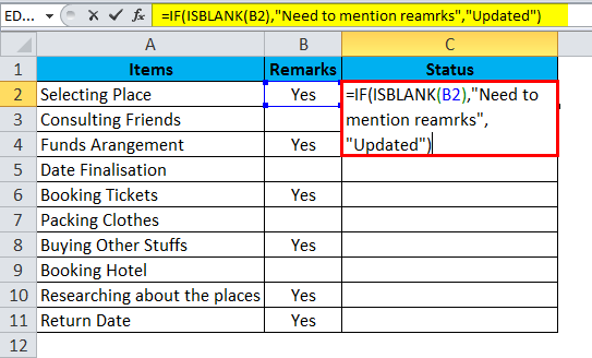
We can track our checklist by using the ISBLANK function. I have a traveling checklist, and if the particular item is already selected, then I have marked that as YES or else blank.
Now I need to identify the status.
I am going to use ISBLKANK with another logical function called IF.
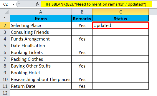
ISBLANK with IF Function returns the status:
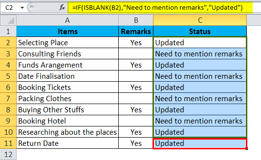
Drag and drop the formula to the remaining cells.
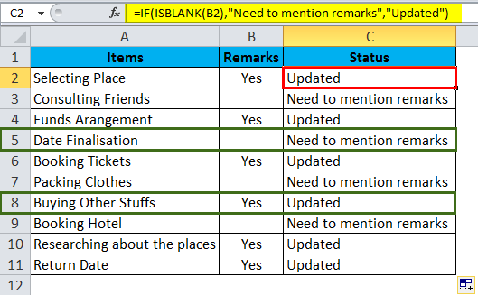
The formula IF checks if the selected cell is blank. If the selected cell is blank, the status will be updated as Needed to mention remarks. If the selected cell is not blank, then the status is updated.
Example #4
We can use the ISBLANK to highlight all the blank cells by using Conditional Formatting.
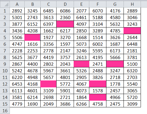
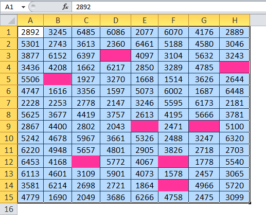
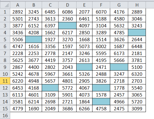
I have a numbers list in the Excel sheet, but it also includes blank cells with pink color.
Step 1: Select the data.
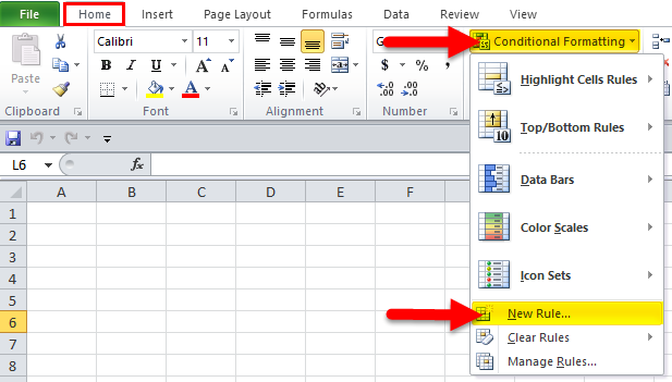
Step 2: Click on Conditional Formatting at the home tab and select a new rule.
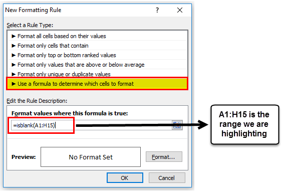
Step 3: Apply the below formula first.
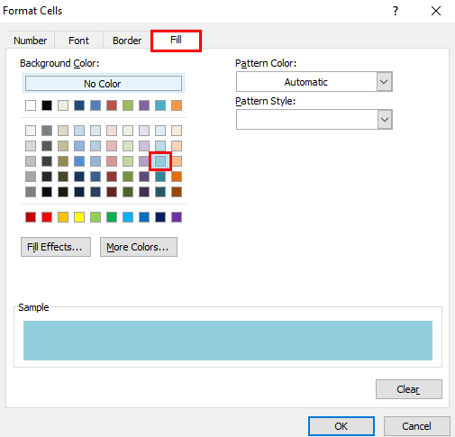
Step 4: Now click on Format and select Fill.
Step 5: Now click on Ok. This would instantly highlight all the blank cells.
Example #5
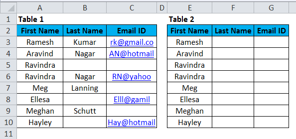
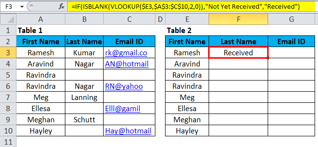
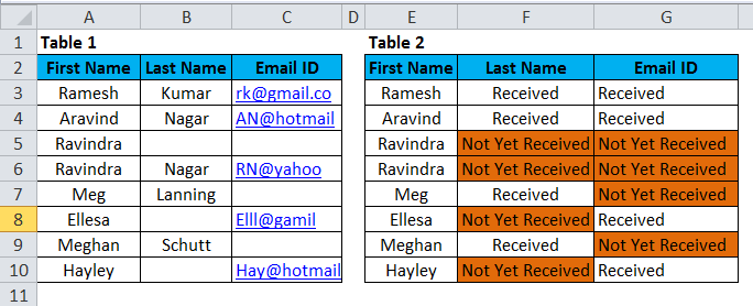
Assume you are collecting the database for your business. Below is the collected data so far. Now the challenge is we do not have all the data. Wherever blank is where we need to find those and mark them as “Not Yet Received”.
Ok, in table 1, I have the actual data. Now I need to pull the data from table 1 and mention it in table 1. If the data is there, I need to mark that as “Received” if “Not Yet Received”.
This can be sorted out using the Vlookup function and the ISBLANK function.
Follow the below steps to learn how to do it.
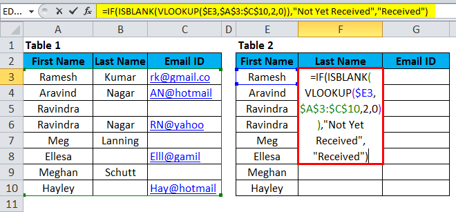
Closely look at the formula here.
=IF (ISBLANK (VLOOKUP ($E4,$A$3:$C$10,2,0)), “Not Yet Received”, “Received”)
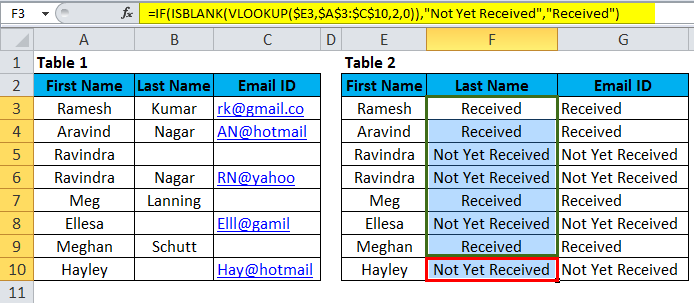
IF formula is checking the value returned by VLOOKUP, is a formula blank or not.
If the value returned by the VLOOKUP formula is not blank, it will return the result as “Received.”
Drag and drop the formula to the remaining cells.
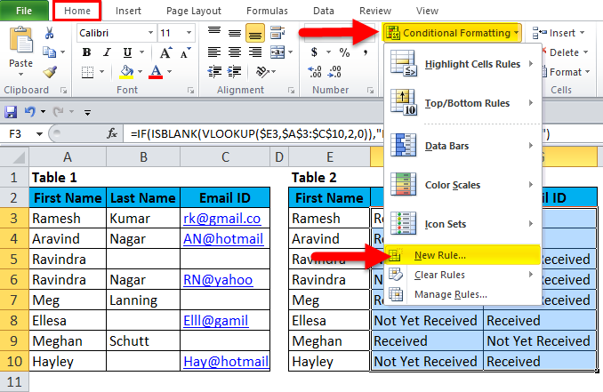
Now highlight all the Not Yet Received results by using Conditional Formatting.
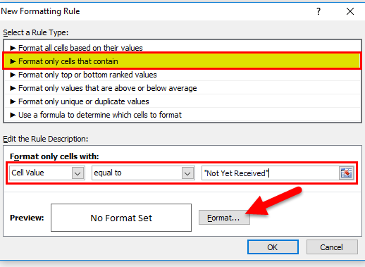
- Select the data and click on Conditional Formatting and New Rule.
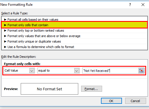
- Select the rule type and edit the Rule description.
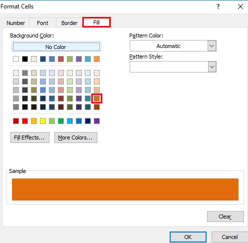
- Now click on Format.
- Select the color you want.
- This would instantly highlight all the “Not Yet Received ” cells.
Things to Remember
- ISBLANK can only find you the blank cells in the cell.
- ISSBLANK can only be applied to a single cell at a time. We cannot select the range of cells for this formula. If you have selected the range of cells, it will read only the first cell as its reference.
- ISBLANK is one of many IS functions in Excel. Other IS functions are ISTEXT, ISERROR, ISNA, ISNUMBER, ISREF, etc…
Recommended Articles
This has been a guide to ISBLANK in Excel. Here we discuss the ISBLANK Formula in Excel and how to use ISBLANK Function in Excel, along with Excel examples and downloadable Excel templates. You may also look at these useful functions in Excel –

