Updated August 24, 2023
ISERROR in Excel
IsError is a simple logical function used for finding if any cell consists of any error statement. And that statement can be #N/A, #Value, #Num, or any other error in MS Excel. So when we use the IsError function, we will only get TRUE if a cell has an error or FALSE if there is no error. An important thing to note about the IsError function is it can only be used in a single cell, and using this function along with other conditional functions will give better results. ISERROR in Excel can help you quickly and easily find errors in your statement.
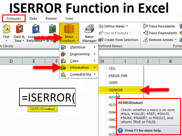
ISERROR finds all the below errors in Excel. Error lists are below.
#N/A, #VALUE!, #REF, #DIV/0!, #NUM!, #NAME?, #NULL!
If the function ISERROR finds any of these in the cell, it will return the result as TRUE or FALSE.
ISERROR Formula in Excel:
The Formula for the ISERROR Function in Excel is as follows:
The Formula of ISERROR includes only one parameter, i.e. value
Value: This is the targeted cell you want to test.
This function is very helpful in replacing the error value with any other value.
How to Use ISERROR Function in Excel?
ISERROR Function in Excel is very simple and easy to use. Let us understand the working of ISERROR in Excel by Some Examples.
Example #1
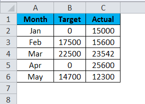
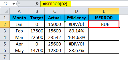
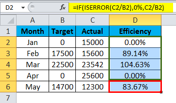
Let’s look at the simple example of the ISERROR Function in Excel. I have target vs actual data from Jan to May.
In column A, I have a month list, in column B, I have a target list, and in column C, I have achieved a list.
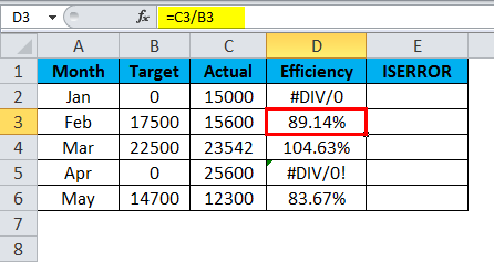
I have calculated the efficiency level by dividing the achieved number by the target number.
The problem is we got some errors as #DIV/0!.
If anyone of the denominator or numerator is zero, we get the error as #DIV/0!When we are dividing numbers.
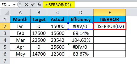
Let me find out which cell has an error value by using the ISERROR function.
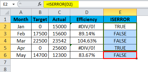
ISERROR Function returns the result as given below:
Since I have applied ISERROR Formula in Excel, it shows as TRUE or else showing as FALSE if there is an error. Drag & drop this function and press CTRL +D for the below values.
However, this is not serving my end purpose. I want the data to be shown as zero if there is an error or else do the normal calculation.
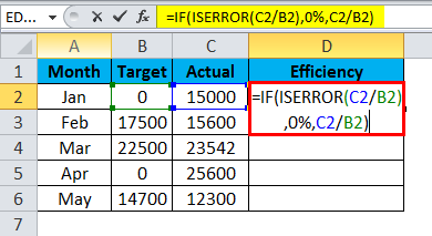
Here I am using the IF condition with the ISERROR function.
A formula I have used here is:
=IF (ISERROR (C2/B2), 0%, C2/B2)
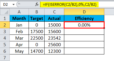
IF condition is checking if the calculation of C2/B2 is returning as an error. If the calculation returning as the error, it will show the result as 0%,.or else do the calculation and show the actual percentage.
Now drag & drop this function and press CTRL +D for the below values.
How cool is it? Showing error values and replacing those error values with the 0% will make the report look beautiful.
Example #2
We have another error function called IFERROR. It works the similar way that ISERROR works, but there is slight modification are there.
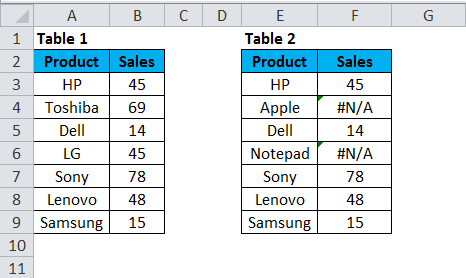
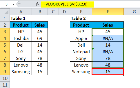
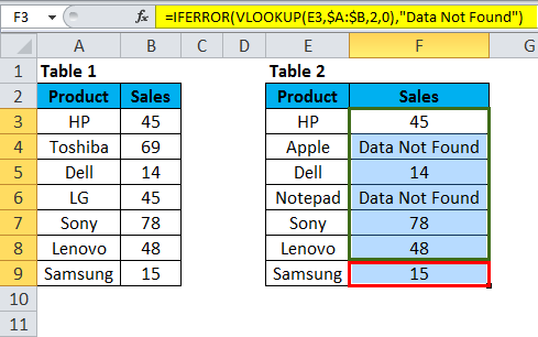
Consider the below example for illustration of the IFERROR function. Table 1 is the main data source, and table 2 is the Vlookup table.
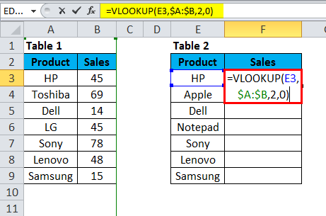
In column F, I have applied the Vlookup formula to find the sales amount for laptop brands.
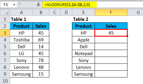
This VLOOKUP Function returns the result as given below:
Now drag & drop this function and press CTRL +D for the below values.
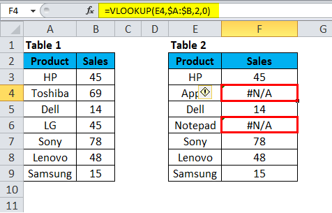
In the above table, I got an error for the brand’s Apple and Notepad. If you look at the main data table, there are no Apple and Notepad brands. That is why Vlookup has returned an error type as #N/A.
We can fix this issue by using the IFERROR Function.
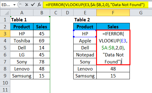
Apply IFEEROR before the VLOOKUP function. We need to write the Vlookup formula inside the IFERROR Formula.
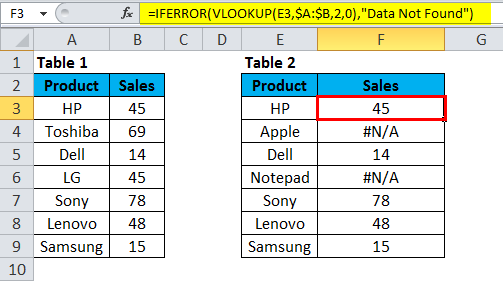
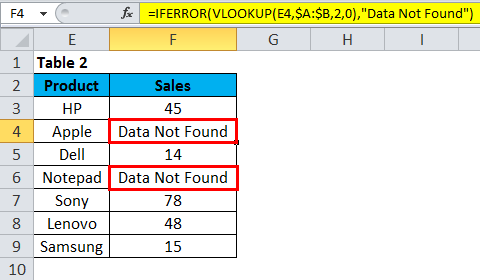
=IFERROR (VLOOKUP (E3, $A: $B, 2, 0),”Data Not Found”). It returns the result as shown below:
Now drag & drop this function and press CTRL +D for the below values.
Firstly, IFERROR trying to find the value for the VLOOKUP formula.
Secondly, If VLOOKUP does not find a value, then it will return an error. Therefore, if there is an error, we will show the result as “Data Not Found”.
We have replaced all the #N/A values with “Data Not Found” text. I think this will look better than the #N/A.
Manual Method for Replacing ERROR Values
However, we can replace the error with ISERROR, IFERROR formula; there is one manual method to do it: the found and replace method.
Step 1: Once the formula is applied and copy and paste only values.
Step 2: Press Ctrl + H to open replace the box and type the error value (#N/A, #DIV/0! etc.). Whatever the error type you want to replace, mention that error.
Step 3: Now write the replace with values as “Data Not Found”.
Step 4: Click on replace all button.
This would instantly replace all the mentioned error values with Data Not Found.
Note: If you have applied filter, please choose visible cells only method to replace.
Things to Remember
- ISERROR can make your numerical reports beautiful by removing all kinds of errors.
- If the data contains an error type and applies pivot tables, then the same kind of error will occur in the Pivot table.
- ISERROR can make the report look beautiful by finding error values and saves you from embarrassments.
- ISERROR can be applied only to one cell at a time. It cannot take many ranges of cells.
- Only the first cell of the range is considered if it is applied to a range of cells.
Recommended Articles
This has been a guide to ISERROR in Excel. Here we discuss the ISERROR Formula in Excel and how to use ISERROR Function in Excel along with excel example and downloadable excel templates. You may also look at these useful functions in excel –
