Updated August 24, 2023
ISNA in Excel
The IsNA function is one of those functions used to find whether a cell has any error. And this only detects one type of error, #N/A which usually occurs when we try to look up any value from the lookup range and that value is not there. So, in the end, we get #N/A which summarizes that the value we want is “Not Available”, and the IsNA function detects if the process would get #N/A or not by returning the TRUE and FALSE statements.
ISNA Formula in Excel:
Below is the ISNA Formula in Excel:
ISNA Formula in Excel has one critical parameter: i.e., value.
- Value (compulsory argument) – The value or expression that needs to be teweightis entered manually or defined variables or a cell reference to use instead.
How to Use the ISNA Function in Excel?
ISNA Function in Excel is very simple and easy to use. Let us understand the working of ISNA Function in Excel by some ISNA Formula in Excel examples.
Example #1 – ISNA Function
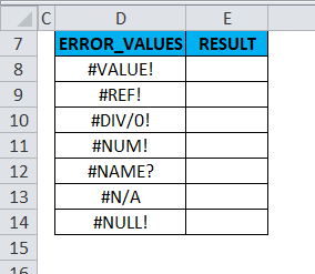
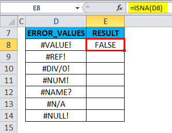
In the below-mentioned table. I have the various error values in the ERROR_VALUES column (column D); here, with the ISNA Function’s help in Excel, I need to find out the #N/A error in column D.
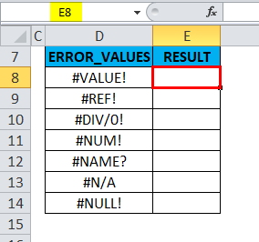
Let’s apply the ISNA function in cell “E8”. Select the cell “E8,” where the ISNA function needs to be applied.
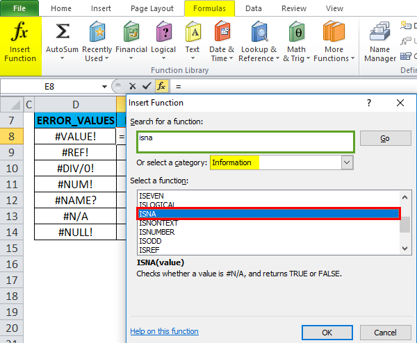
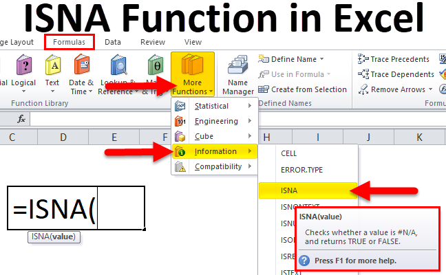
Click the insert function button (fx) under the formula toolbar; a dialog box will appear, type the keyword “ISNA” in the search for a function box & under select a category dropdown, select “INFORMATION” so that the ISNA function will appear in select a Function box. Double click on ISNA Function.
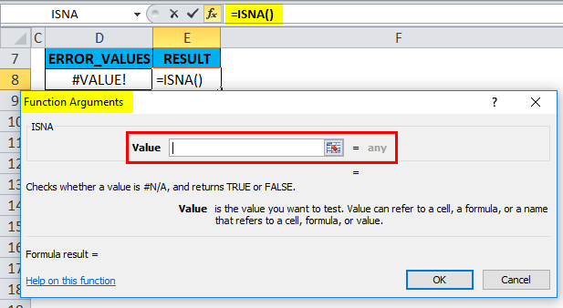
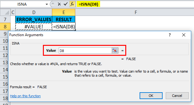
A dialog box appears where arguments for ISNA Function need to be filled or entered, i.e., =ISNA(value)
Value: Here, I have to check whether the value in cell D8 contains the #N/A error. I must mention the cell reference “D8”, i.e., =ISNA(D8).
Here, =ISNA(D8) will return TRUE if the value is an #N/A error or return FALSE if it doesn’t contain a #N/A error.
Cell D8 does not contain the #N/A error; it will return FALSE as an output in cell “E8”.
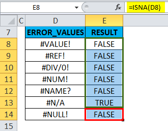
To get the output for the complete dataset, click inside cell E8 to see the cell selected, then Select the cells till E14. Once it got selected, the column range will get selected; click on Ctrl + D so that the ISNA formula is applied to the whole range.
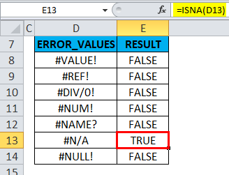
E13 cell returns TRUE value because the D13 cell contains #N/A Error.
Example #2 – ISNA & IF Function with VLOOKUP Function to Avoid #N/A Error
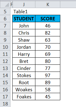
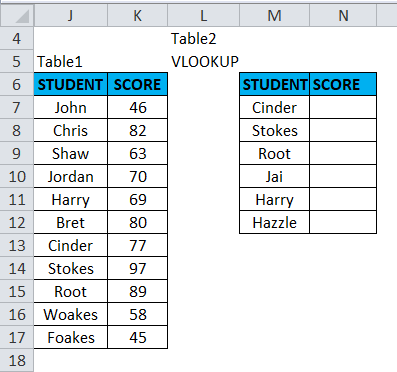
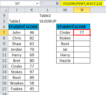
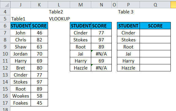
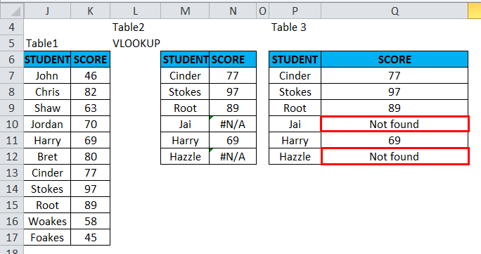
In the below-mentioned table1. I have the list of students in the Student column (Column J) & their scores in the Score column (Column K).
Table 2 contains a list of student names in the student column (column M); our objective here in this table is to find the student’s score based on his name, i.e., student name (refer to table 1), by using the VLOOKUP Function.
Before applying a VLOOKUP formula, You should be aware of it. Vertical lookup or VLOOKUP references vertically aligned tables and quickly finds data in relation to the value the user enters.
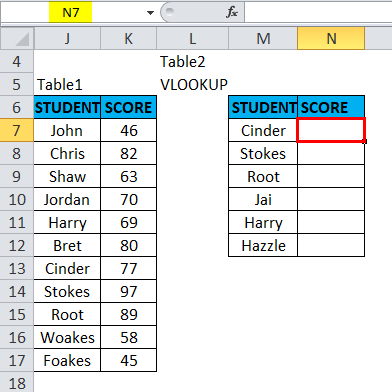
Let’s apply VLOOKUP Function in cell “N7”. Select the cell “N7” where VLOOKUP Function needs to be applied.
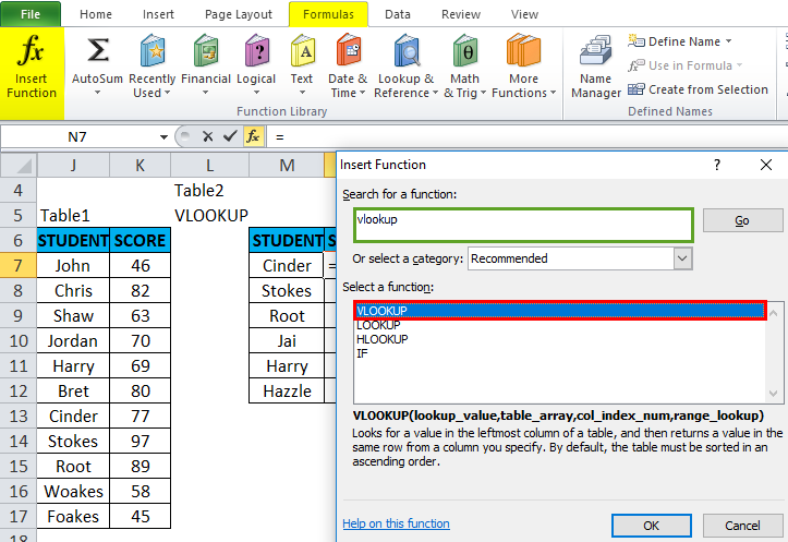
Click the insert function button (fx) under the formula toolbar; a dialog box will appear, type the keyword “VLOOKUP” in the search for a function box; VLOOKUP Function will appear in the select a Function box. Double click on the VLOOKUP function.
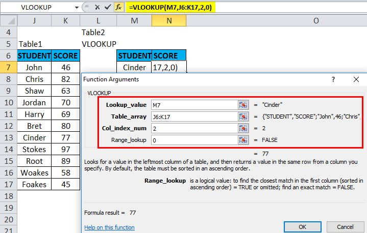
A dialog box appears where arguments for the VLOOKUP function need to be filled or entered.
The syntax for the VLOOKUP function is:
VLOOKUP (lookup_value, table_array, col_index_num, [range_lookup])
- lookup_value: the value you want to look up, i.e., “M7” or “CINDER”.
- table_array: range where the lookup value is located, i.e., select table1 range J6:K17.
- col_index_num: column number in a table array from which the matching value should be returned. The student score in Table 1 is in the second column, i.e., 2.
- range_lookup: FALSE for an exact match or TRUE for an approximate game. Select 0 or false.
=VLOOKUP(M7, J6:K17,2,0) returns the score of cinder, i.e., 77.
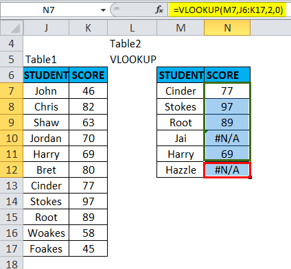
To get the finalized data for other students, click inside cell N7 to see the cell selected, then Select the cells till N12. Once it got selected, the column range will be selected; click on Ctrl + D so that the VLOOKUP formula is applied to the whole range.
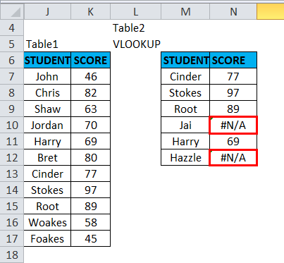
Here, the #N/A error is returned in cells N10 & N12 because the Vlookup function fails to find a match to the supplied lookup_value in the reference table range.
#N/A error looks odd for a better outlook of a final dataset without a N/A error. ISNA function is used with the IF function in the VLOOKUP function to avoid the #N/A error, where the #N/A error value is replaced with a customized text string.
Suppose I want a customized message, i.e., “Not found” instead of the #N/A error.
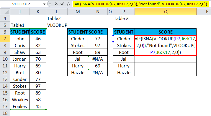
Let’s work on this in Table 3; below mentioned ISNA function with IF is used with the VLOOKUP function to avoid the #N/A error.
=IF(ISNA(VLOOKUP(P7,J6:K17,2,0)),”Not found”,VLOOKUP(P7,J6:K17,2,0))
Three parts of the formula are
- =IF(ISNA(VLOOKUP(P7,J6:K17,2,0)),
The first part of the formula means if the function doesn’t find the value of cell P7 in table range J6:K17, then display the second part.
- “Not found.”
Display “Not found” instead of a #N/A.
- VLOOKUP(P7,J6:K17,2,0))
If the function finds the value, perform the VLOOKUP formula as usual.
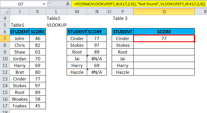
Let’s apply this formula in cell “Q7”.
The Result will be :
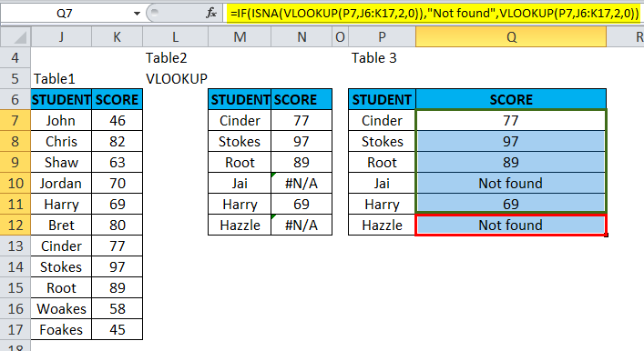
We need to apply this formula for a whole date range to get the finalized data for other students. Click inside cell “Q7” to see the cell selected; then Select the cells until Q12. Once it gets selected, the column range will get selected; click on Ctrl + D to apply the formula to the whole range.
It will return a customized text string mentioned in the formula, i.e., “Not found” instead of the #N/A error in the cell N10 & N12.
Things to Remember about the ISNA Function in Excel
- ISNA argument value can be a blank (empty cell), text, number, error, logical, or reference value, or a name referring to any of these you want to test.
- IS functions are significant in formulas for testing the outcome of a calculation. If it is combined with IF logical conditions, it will help out to find the error value.
Recommended Articles
This has been a guide to ISNA in Excel. Here we discuss the ISNA Formula in Excel and How to use ISNA Function in Excel, along with practical examples and a downloadable Excel template. You can also go through our other suggested articles –

