Updated May 30, 2023
Introduction to Jacobian Matlab
Jacobian is a determinant defined for a finite number of input functions and the same limited number of variables. Each row of Jacobian will consist of each variable’s 1st partial derivatives of the input function w.r.t. In this topic, we are going to learn about Jacobian Matlab.
In MATLAB, Jacobian is mainly of 2 types:
- Vector function’s Jacobian: It is a matrix with partial derivatives of the input vector function.
- Scalar function’s Jacobian: For a scalar function, Jacobian gives transpose of the input function’s gradient.
We use the Jacobian function in MATLAB to get the Jacobian matrix.
Syntax:
jacobian (F, Z)
Description:
jacobian (F, Z) is used to get the Jacobian matrix for input function ‘F’ w.r.t Z.
Examples of Jacobian Matlab
Let us now understand the code to get the Jacobian matrix in MATLAB using different examples:
Example #1
In this example, we will take a vector function and will compute its Jacobian Matrix using the Jacobian function. For our first example, we will input the following values:
- Pass the input vector function as [b*a, a + c, b^3]
- Pass the variables as [a, b, c]
Code:
syms a b c

[Initializing the variables ‘a’, ‘b’, ‘c’]
jacobian ([b*a, a+c, b^3], [a, b, c])

[Passing the input vector function and variables as the arguments]
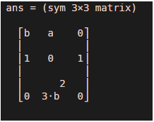
* Mathematically, the Jacobian matrix of [b*a, a+c, b^3] concerning [a, b, c] is

[ b, a, 0]
[ 1, 0, 1]
[ 0, 3*b^2, 0]
Input:
syms a b c

jacobian ([b*a, a+c, b^3], [a, b, c])
Output
As we can see in the output, we have obtained a partial derivative of every element of the input vector function w.r.t each variable passed as input.
Example #2
In this example, we will take another vector function and will compute its Jacobian Matrix using the Jacobian function. For this example, we will input the following values:
- Pass the input vector function as [a^4 + b, a^2 + c, b + 3]
- Pass the variables as [a, b, c]
Code:
syms a b c

[Initializing the variables ‘a’, ‘b’, ‘c’]
jacobian([a^4 + b, a^2 + c, b + 3], [a, b, c])

[Passing the input vector function and variables as the arguments]
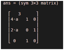
* Mathematically, the Jacobian matrix of [a^4 + b, a^2 + c, b + 3]with respect to [a, b, c] is

[ 4*a^3,   1,   0]
[   2*a,     0,   1]
[     0,       1,   0]
Input:
syms a b c

jacobian([a^4 + b, a^2 + c, b + 3], [a, b, c])
Output:
As we can see in the output, we have obtained a partial derivative of every element of the input vector function w.r.t each variable passed as input.
Example #3
In this example, we will take another vector function and will compute its Jacobian Matrix using the Jacobian function. For this example, we will input the following values:
- Pass the input vector function as [c^3 + b^2, 2*a^3 + c, c^2 + 5]
- Pass the variables as [a, b, c]
Code:
syms a b c

[Initializing the variables ‘a’, ‘b’, ‘c’]
jacobian([c^3 + b^2, 2*a^3 + c, c^2 + 5], [a, b, c])

[Passing the input vector function and variables as the arguments]
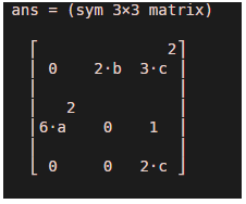
* Mathematically, the Jacobian matrix of [c^3 + b^2, 2*a^3 + c, c^2 + 5] with respect to [a, b, c] is

[     0,          2*b,   3*c^2]
[ 6*a^2,     0,        1]
[     0,          0,        2*c]
Input:
syms a b c

jacobian([c^3 + b^2, 2*a^3 + c, c^2 + 5], [a, b, c])
Output:
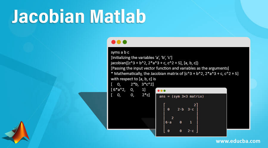
As we can see in the output, we have obtained a partial derivative of every element of the input vector function w.r.t each variable passed as input.
Next, let us take a few examples to understand the Jacobian function in the case of Scalars.
Example #4
In this example, we will take a scalar function and will compute its Jacobian Matrix using the Jacobian function. For our first example, we will input the following values:
- Pass the input scalar function as 3*a^2 + c*b^3 + a^2
- Pass the variables as [a, b, c],
Code:
syms a b c

[Initializing the variables ‘a’, ‘b’, ‘c’]
jacobian(3*a^2 + c*b^3 + a^2, [a, b, c])

[Passing the input scalar function and variables as the arguments]
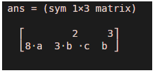
* Mathematically, the Jacobian matrix of 3*a^2 + c*b^3 + a^2 concerning [a, b, c] is

[ 8*a, 3*b^2*c, b^3, 0]
Input:
syms a b c

jacobian(3*a^2 + c*b^3 + a^2, [a, b, c])
Output:
As we can see in the output, we have obtained transpose of the gradient as the Jacobian matrix for a scalar function.
Example #5
In this example, we will take another scalar function and will compute its Jacobian Matrix using the Jacobian function. For our first example, we will input the following values:
- Pass the scalar input function as b^4 + a^3 – c*d
- Pass the variables as [a, b, c, d],
Code:
syms a b c d

[Initializing the variables ‘a’, ‘b’, ‘c’, ‘d’]
jacobian(b^4 + a^3 - c*d, [a, b, c, d])

[Passing the input scalar function and variables as the arguments]
* Mathematically, the Jacobian matrix of b^4 + a^3 -c*d concerning [a, b, c, d] is

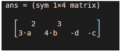
[ 3*a^2, 4*b^3, -d, -c]
Input:
syms a b c d

jacobian(b^4 + a^3 - c*d, [a, b, c, d])
Output:
As we can see in the output, we have obtained transpose of the gradient as the Jacobian matrix for a scalar function.
Conclusion
The jacobian function is used in MATLAB to find the Jacobian matrix of any function (vector or scalar). For a scalar, the Jacobian function provides us with the transpose of the gradient for the scalar function.
Recommended Articles
This is a guide to Jacobian Matlab. Here we discuss the Jacobian matrix in MATLAB using different examples along with the sample codes. You may also have a look at the following articles to learn more –
