Updated March 20, 2023

Introduction to Kernel Methods
Kernels or kernel methods (also called Kernel functions) are sets of different types of algorithms that are being used for pattern analysis. They are used to solve a non-linear problem by using a linear classifier. Kernels Methods are employed in SVM (Support Vector Machines) which are used in classification and regression problems. The SVM uses what is called a “Kernel Trick” where the data is transformed and an optimal boundary is found for the possible outputs.
The Need for Kernel Method and its Working
Before we get into the working of the Kernel Methods, it is more important to understand support vector machines or the SVMs because kernels are implemented in SVM models. So, Support Vector Machines are supervised machine learning algorithms that are used in classification and regression problems such as classifying an apple to class fruit while classifying a Lion to the class animal.
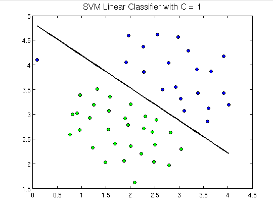
To demonstrate, below is what support vector machines look like:
Here we can see a hyperplane which is separating green dots from the blue ones. A hyperplane is one dimension less than the ambient plane. E.g. in the above figure, we have 2 dimension which represents the ambient space but the lone which divides or classifies the space is one dimension less than the ambient space and is called hyperplane.
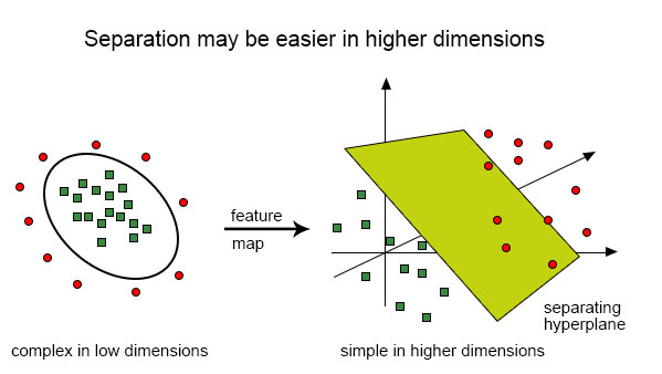
But what if we have input like this:
It is very difficult to solve this classification using a linear classifier as there is no good linear line that should be able to classify the red and the green dots as the points are randomly distributed. Here comes the use of kernel function which takes the points to higher dimensions, solves the problem over there and returns the output. Think of this in this way, we can see that the green dots are enclosed in some perimeter area while the red one lies outside it, likewise, there could be other scenarios where green dots might be distributed in a trapezoid-shaped area.
So what we do is to convert the two-dimensional plane which was first classified by one-dimensional hyperplane (“or a straight line”) to the three-dimensional area and here our classifier i.e. hyperplane will not be a straight line but a two-dimensional plane which will cut the area.
In order to get a mathematical understanding of kernel, let us understand the Lili Jiang’s equation of kernel which is:
K(x, y)=<f(x), f(y)> where,
K is the kernel function,
X and Y are the dimensional inputs,
f is the map from n-dimensional to m-dimensional space and,
< x, y > is the dot product.
Illustration with the help of an example.
Let us say that we have two points, x= (2, 3, 4) and y= (3, 4, 5)
As we have seen, K(x, y) = < f(x), f(y) >.
Let us first calculate < f(x), f(y) >
f(x)=(x1x1, x1x2, x1x3, x2x1, x2x2, x2x3, x3x1, x3x2, x3x3)
f(y)=(y1y1, y1y2, y1y3, y2y1, y2y2, y2y3, y3y1, y3y2, y3y3)
so,
f(2, 3, 4)=(4, 6, 8, 6, 9, 12, 8, 12, 16)and
f(3 ,4, 5)=(9, 12, 15, 12, 16, 20, 15, 20, 25)
so the dot product,
f (x). f (y) = f(2,3,4) . f(3,4,5)=
(36 + 72 + 120 + 72 +144 + 240 + 120 + 240 + 400)=
1444
And,
K(x, y) = (2*3 + 3*4 + 4*5) ^2=(6 + 12 + 20)^2=38*38=1444.
This as we find out, f(x).f(y) and K(x, y) give us the same result, but the former method required a lot of calculations(because of projecting 3 dimensions into 9 dimensions) while using the kernel, it was much easier.
Types of Kernel and methods in SVM
Let us see some of the kernel function or the types that are being used in SVM:
1. Liner Kernel
Let us say that we have two vectors with name x1 and Y1, then the linear kernel is defined by the dot product of these two vectors:
K(x1, x2) = x1 . x2
2. Polynomial Kernel
A polynomial kernel is defined by the following equation:
K(x1, x2) = (x1 . x2 + 1)d,
Where,
d is the degree of the polynomial and x1 and x2 are vectors
3. Gaussian Kernel
This kernel is an example of a radial basis function kernel. Below is the equation for this:
The given sigma plays a very important role in the performance of the Gaussian kernel and should neither be overestimated and nor be underestimated, it should be carefully tuned according to the problem.
4. Exponential Kernel
This is in close relation with the previous kernel i.e. the Gaussian kernel with the only difference is – the square of the norm is removed.
The function of the exponential function is:
This is also a radial basis kernel function.
5. Laplacian Kernel
This type of kernel is less prone for changes and is totally equal to previously discussed exponential function kernel, the equation of Laplacian kernel is given as:
6. Hyperbolic or the Sigmoid Kernel
This kernel is used in neural network areas of machine learning. The activation function for the sigmoid kernel is the bipolar sigmoid function. The equation for the hyperbolic kernel function is:
This kernel is very much used and popular among support vector machines.
7. Anova radial basis kernel
This kernel is known to perform very well in multidimensional regression problems just like the Gaussian and Laplacian kernels. This also comes under the category of radial basis kernel.
The equation for Anova kernel is :
There are a lot more types of Kernel Method and we have discussed the mostly used kernels. It purely depends on the type of problem which will decide the kernel function to be used.
Conclusion
In this section, we have seen the definition of the kernel and how it works. We tried to explain with the help of diagrams about the working of kernels. We have then tried to give a simple illustration using math about the kernel function. In the final part, we have seen different types of kernel functions that are widely used today.
Recommended Articles
This is a guide to Kernel Methods. Here we discuss an introduction, need, it’s working and types of kernel methods with the appropriate equation. You can also go through our other suggested articles to learn more –


