Updated March 21, 2023

Overview of Linear Regression Modeling
Linear Regression has actually been around for a very long time (around 200 years). It is a linear model, i.e. it assumes a linear relationship between the input variables(x) and a single output variable(y). The y here is calculated by the linear combination of the input variables.
Linear regression is a type of machine learning algorithm that is used to model the relation between scalar dependent and one or more independent variables. The case of having one independent variable is known as simple linear regression, while the case of having multiple linear regression is known as multiple linear regression. In both of these linear regressions, the model is constructed using a linear predictor function. The unknown data parameters are estimated using the available dataset because this feature has various applications such as finance, economics, epidemiology, etc.
Hence, supervised Learning is the learning where we train the machine to understand the relationship between the input and output values provided in the training data set and then use the same model to predict the output values for the testing data set. So, basically, if we have the output or labeling already provided in our training data set and we are sure that the output provided makes sense corresponding to the input, then we use Supervised Learning. Supervised learning algorithms are classified into Regression and Classification.
Regression algorithms are used when you notice that the output is a continuous variable, whereas classification algorithms are used when the output is divided into sections such as Pass/Fail, Good/Average/Bad, etc. We have various algorithms for performing the regression or classification actions, with Linear Regression Algorithm being the basic algorithm in Regression.
Coming to this Regression, before getting into the algorithm, let me set the base for you. In schooling, I hope you remember the line equation concept. Let me give a brief about it. You were given two points on the XY plane, i.e. say (x1,y1) and (x2,y2), where y1 is the output of x1 and y2 is the output of x2, then the line equation that passes through the points is (y-y1)=m(x-x1) where m is the slope of the line. After finding the line equation, if you are given a point, say (x3,y3), you would be easily able to predict if the point lies on the line or the distance of the point from the line. This was the basic regression that I had done in schooling without even realizing that this would have such great importance in Machine Learning. We generally do in this to identify the equation line or curve that could fit the input and output of the train data set properly and then use the same equation to predict the output value of the test data set. This would result in a continuous desired value.
Two Types of Linear Regression
Let’s talk about two types of Linear Regression.
1. Simple Linear Regression
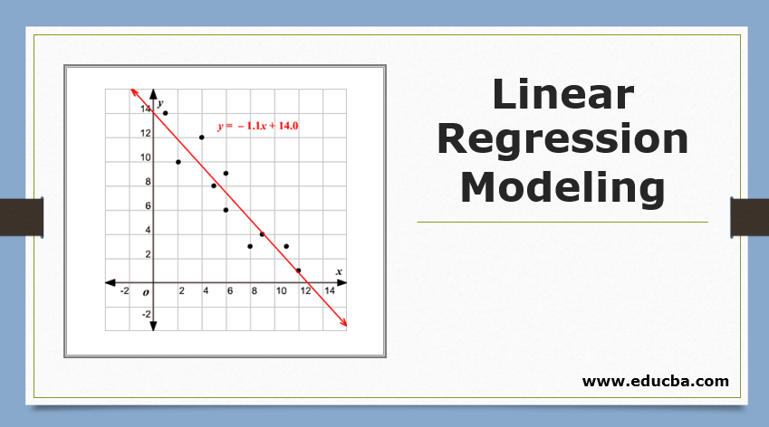
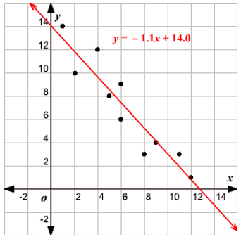
When there is a single input variable, i.e. line equation is c
considered as y=mx+c, then it is Simple Linear Regression.
2. Multiple Linear Regression
When there are multiple input variables, i.e. line equation is considered as y = ax1+bx2+…nxn, then it is Multiple Linear Regression. Various techniques are utilized to prepare or train the regression equation from data, and the most common one among them is called Ordinary Least Squares. The model built using the mentioned method is referred to as Ordinary Least Squares Linear Regression or just Least Squares Regression. Model is used when the input values and the output value to be determined are numeric values. When there are only one input and one output, then the equation formed is a line equation i.e.
y = B0x+B1
where the coefficients of the line are to be determined using statistical methods.
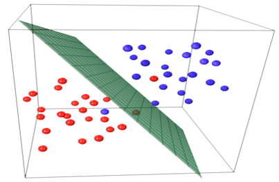
Simple Linear Regression models are rare in ML because we will generally have various input factors to determine the outcome. When there are multiple input values and one output value, then the equation formed is that of a plane or hyper-plane.
y = ax1+bx2+…nxn

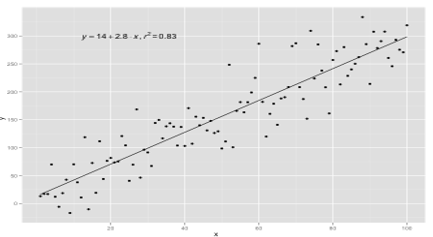
The core idea in the regression model is to obtain a line equation that best fits the data. The best fit line is when the total prediction error for all the data points is considered as small as possible. The error is the distance between the point on the plane to the regression line.
Example
Let us start with an example of Simple Linear Regression.
The relationship between the height and weight of a person is directly proportional. A study has been performed on the volunteers to determine the height and ideal weight of the person, and the values have been recorded. This will be considered as our training data set. Using the training data, a regression line equation is calculated, which will give a minimum error. This linear equation is then used for making predictions on new data. That is, if we give the height of the person, then the corresponding weight should be predicted by the model developed by us with minimum or zero error.
Y(pred) = b0 + b1*x
The values b0 and b1 must be chosen so that they minimize the error. If the sum of squared error is taken as a metric to evaluate the model, then the goal to obtain a line that best reduces the error.
We are squaring out the error so that positive and negative values will not cancel out each other. For model with one predictor:
Calculation of Intercept (b0) in the line equation is done by:
Calculation of the coefficient for the input value x is done by:
Understanding the coefficient b1:
- If b1 > 0, then x(input) and y(output) are directly proportional. That is, an increase in x will increase y, such as height increases, weight increases.
- If b1 < 0, then x(predictor) and y(target) are inversely proportional. That is, an increase in x will decrease y, such as the speed of a vehicle increase, time is taken decreases.
Understanding the coefficient b0:
- B0 takes up the residual value for the model and ensures that the prediction is not biased. If we have not B0 term, then the line equation (y=B1x) is forced to pass through the origin, i.e. the input and output values put into the model result in 0. But this will never be the case; if we have 0 in input, then B0 will be the average of all predicted values when x=0. Setting all predictor values to be 0 in the case of x=0 will result in data loss and is often impossible.
Apart from the coefficients mentioned above, this model can also be calculated using normal equations. I will discuss further the use of normal equations and designing a simple/multilinear regression model in my upcoming article.
Recommended Articles
This is a guide to Linear Regression Modeling. Here we discuss the basic concept, Types of Linear Regression which includes Simple and Multiple Linear Regression along with some examples. You may also look at the following articles to learn more–


