Updated August 11, 2023
Excel Column Lock (Table of Contents)
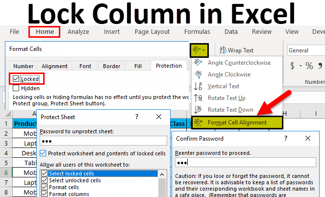
Lock Column in Excel
To lock a column in Excel, we first need to select the column we need to Lock. Then click right anywhere on the selected column and select the Format Cells option from the right-click menu list. Now from the Protection tab of Format Cells, check the box of LOCKED with a tick. There is another way to lock a column which can be done using the Protect Sheet option available under the Review menu tab. First, select the column which wants to lock, then use Protect Sheet with a password to lock it.
How to Lock Column in Excel?
To Lock a column in excel is very simple and easy. Let’s understand how to Lock Columns in Excel with some examples.
Example #1
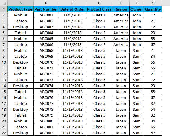
We got sample sales data from some products. Where we have observed that the Product Type column many times got changed by multiple logins. So, to avoid this, we are going to lock that Product Type column so that no one will change it. And data available after it will be accessible for changes. Below is the screenshot of available data for locking the required column.
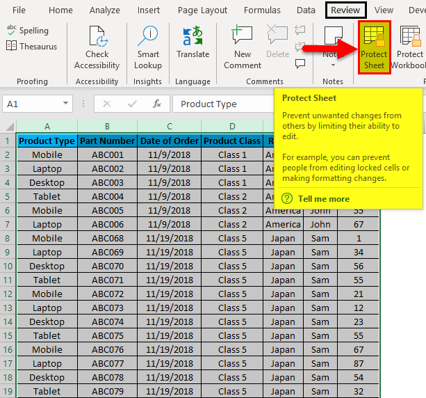
- For this purpose, first, select a cell or column which we need to protect, and then go to the Review tab and click on Protect Sheet.
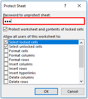
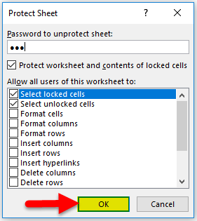
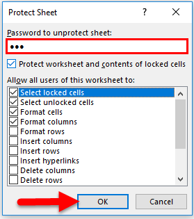
- Once we click on Protect Sheet, we will get a dialog box of Protect Sheet where we need to set a Password of any digit. Here we have set the password as 123.
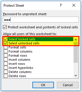
- And check (tick) the options available in a box as per requirement. For example, I have checked selective locked cells and selected unlocked cells (which sometimes comes as default).
- Once we are done with selecting the options for protecting the sheet or column, click on OK as highlighted below.
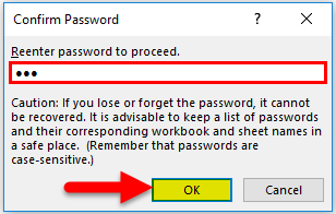
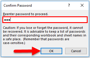
- Once clicked on OK, the system will ask you to re-enter the password again. Once fed the password, click OK.
Now selected Column is locked, and no one can change anything in it without disabling the column’s protection.
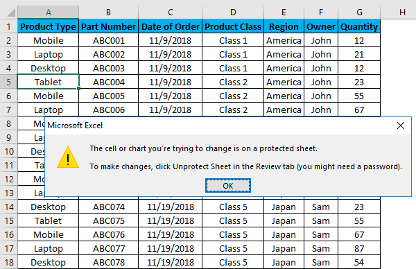
Let’s check whether the column is actually protected now. We had chosen Column A named as Product Type as required. For checking it, try to go in edit mode for any cell of that column (By Pressing F2 or double click); if it is protected, we will see a warning message as below.
Hence, our column data is now protected successfully.
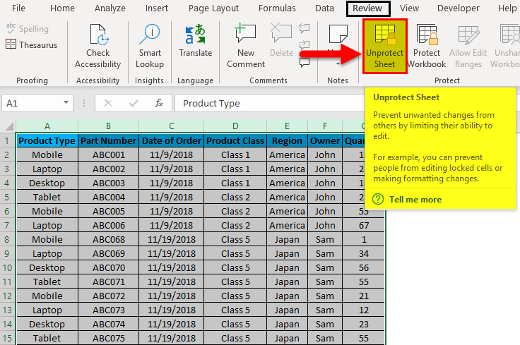
For unprotecting it again, go to the Review tab and click on the Unprotect Sheet, as shown below.
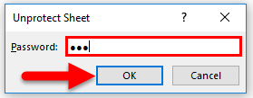
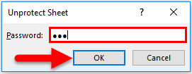
Once we click on the Unprotect Sheet, it will again ask for the same password to unprotect it. For that, re-enter the same password and click on Ok.
Now the column is unprotected, and we can make changes to it. We can also check the column whether it is accessible or not.
Example #2
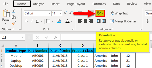
Apart from the method which we have seen in the above example, we can lock any column in excel by this too. In this method, we will lock the desired column by using the Format Cell in Excel. If you are using this function for the first time, you will see your entire sheet selected as Locked to check-in Format cell. For that, select the entire sheet and go to the Home menu and Click the Orientation icon as shown below.
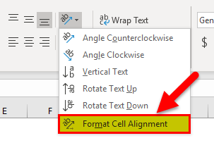
After that, a drop-down will appear. From there, click on Format Cell Alignment, as shown below.
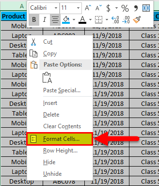
Format Cell Alignment can be accessed from different methods as well. This one is a shortcut approach for doing it. For this, select the entire sheet and Right Click anywhere. We will have the Format Cells option from right-click menu, as shown in the below screenshot. Click on it.
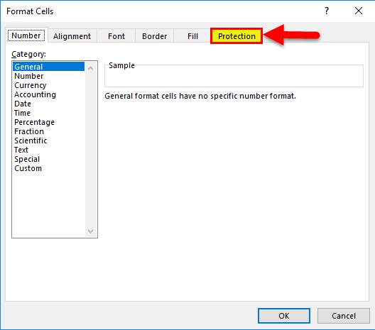
Once we click on it, we will get a dialog box of Format Cell. From there, go to the Protection tab.
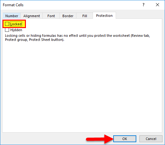
If you find the Locked box is already checked in (which is the default set), then uncheck it click on OK as shown below.
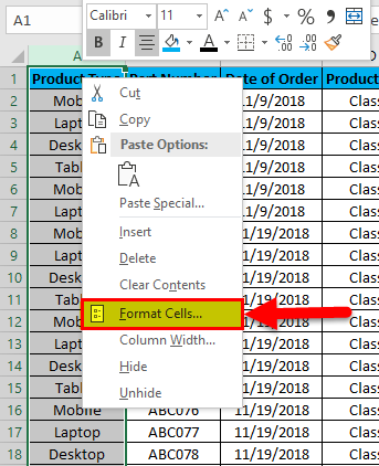
By doing this, we are clearing the default setting and customizing the sheet/column to protect it. Now select the column which we want to lock in excel. Here we are locking column A named as Product Type. Right-click on the same column, and select the Format Cell option.
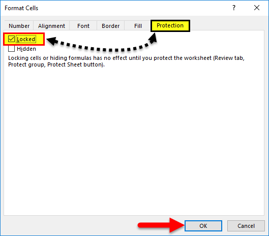
After that, we will see the Format Cell box; go to the Protection Tab and Check-in Locked box. And again, click on OK, as shown below.
Follow the same procedure as explained in example-1. Refer to the below screenshot.
Re-enter the password and click on Ok.
For checking, we already chosen Column A named as Product Type as most of the time, the data available in Product Type gets disturbed. If it is protected, we will see a warning message as below.
So, we will have our column data protected and locked for making any changes.
For unprotecting it again, follow the same procedure as explained in example-1, as shown below.
Once we click on the Unprotect Sheet, it will again ask for the same password to unprotect it. For that, re-enter the same password and click on OK.
Now the column is unprotected, and we can make changes to it. We can also check the column whether it is accessible or not.
Pros of Excel Column Lock
- It helps in data protection by not allowing any unauthorized person to make any changes.
- Sometimes data is so confidential that, even if a file is shared with someone outside the company, then also a person will not be able to do anything, as the sheet/column is locked.
Cons of Excel Column Lock
- Sometimes sheet gets so locked that, even in an emergency, we would not be able to change anything.
- If we forget the password, then also there is no way to make changes in data. There will be only one way to create a new file with the same data to proceed further.
Things to Remember
- Always note the password if you cannot remember it in the long future use.
- Always have a backup of the file which is locked, without any password, so that it will be used further.
- There are no criteria for creating a password.
Recommended Articles
This has been a guide to Lock Column in Excel. Here we discuss how to Lock Columns in Excel along with practical examples and a downloadable Excel template. You can also go through our other suggested articles –
