Updated June 8, 2023
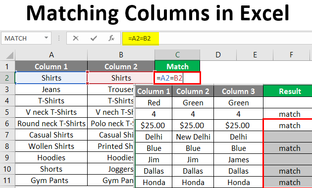
Matching Columns in Excel (Table of Contents)
Introduction to Matching Columns in Excel
Many a time in Excel, we have to compare two columns. There are different techniques for that. We can use IF, COUNTIFS, Match, and conditional formatting functions. We can find the matching data in both the columns and the different ones.
There are various examples of matching columns with different functions. Using any of them per the requirement will give you matching data in two or more columns.
Comparing Two Columns Row by Row
This is one of the basic comparisons of data in two columns. In this, the data is compared row by row to find the matching and difference in data.
How to Match Columns in Excel?
Matching Columns in Excel is very simple and easy. Let’s understand how to use the Matching Columns in Excel with some examples.
Example #1 – Comparing Cells in Two Columns
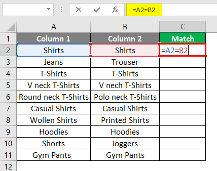
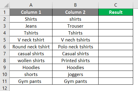
Let’s compare cells in two columns that are in the same row. Below is a table with two columns with some data, which can be the same or different. We can find the similarity and the differences in data as shown below.
Now we will type =A2=B2 in cell C2.
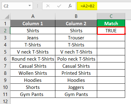
After using the formula result shown below in cell C2.
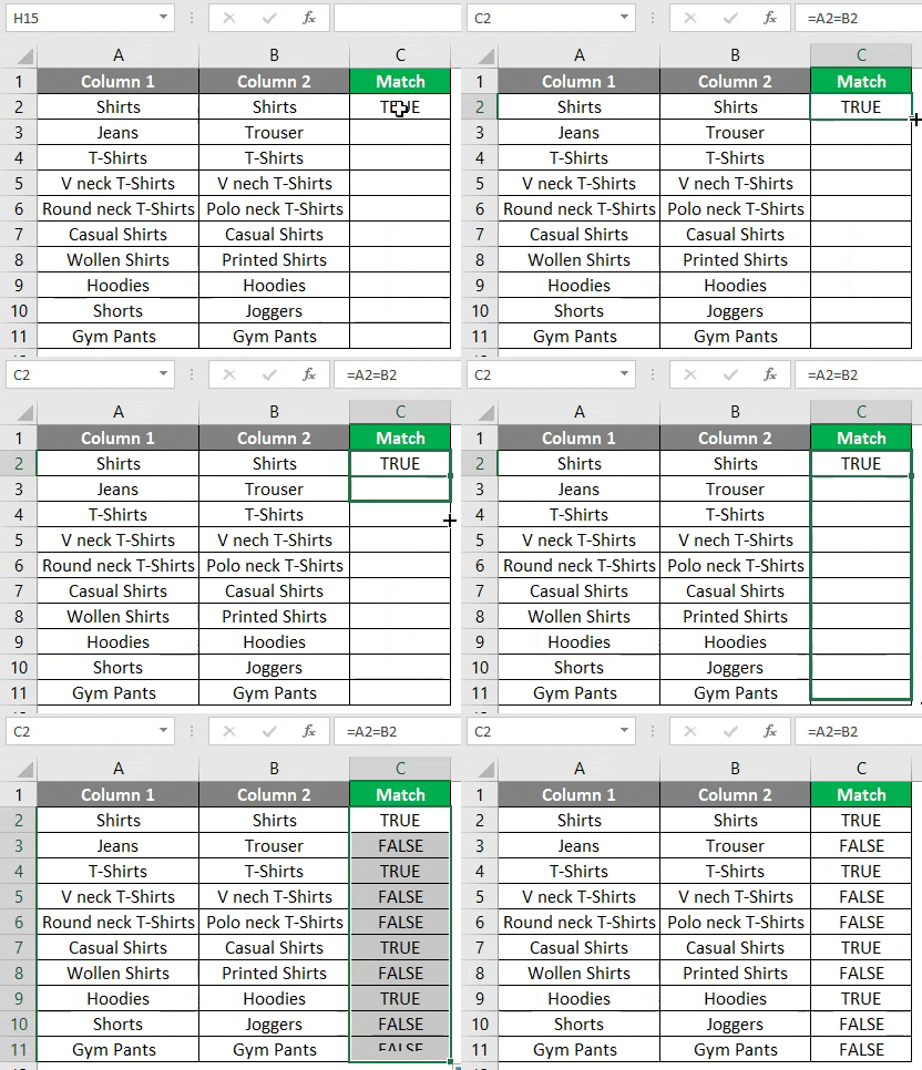
And then drag it downwards to get the result.
Matching cells are giving “True” and different ones “False”.
Example #2 – Comparing Two Cells in the Same Row
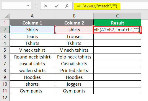
Let’s compare two cells in the same row using the IF function.
We can write the IF formula in cell C2 using our data table.
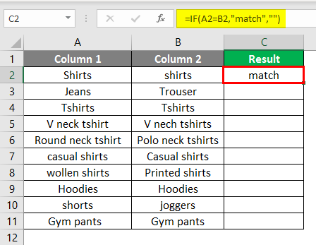
After using the IF Formula, the result is shown below.
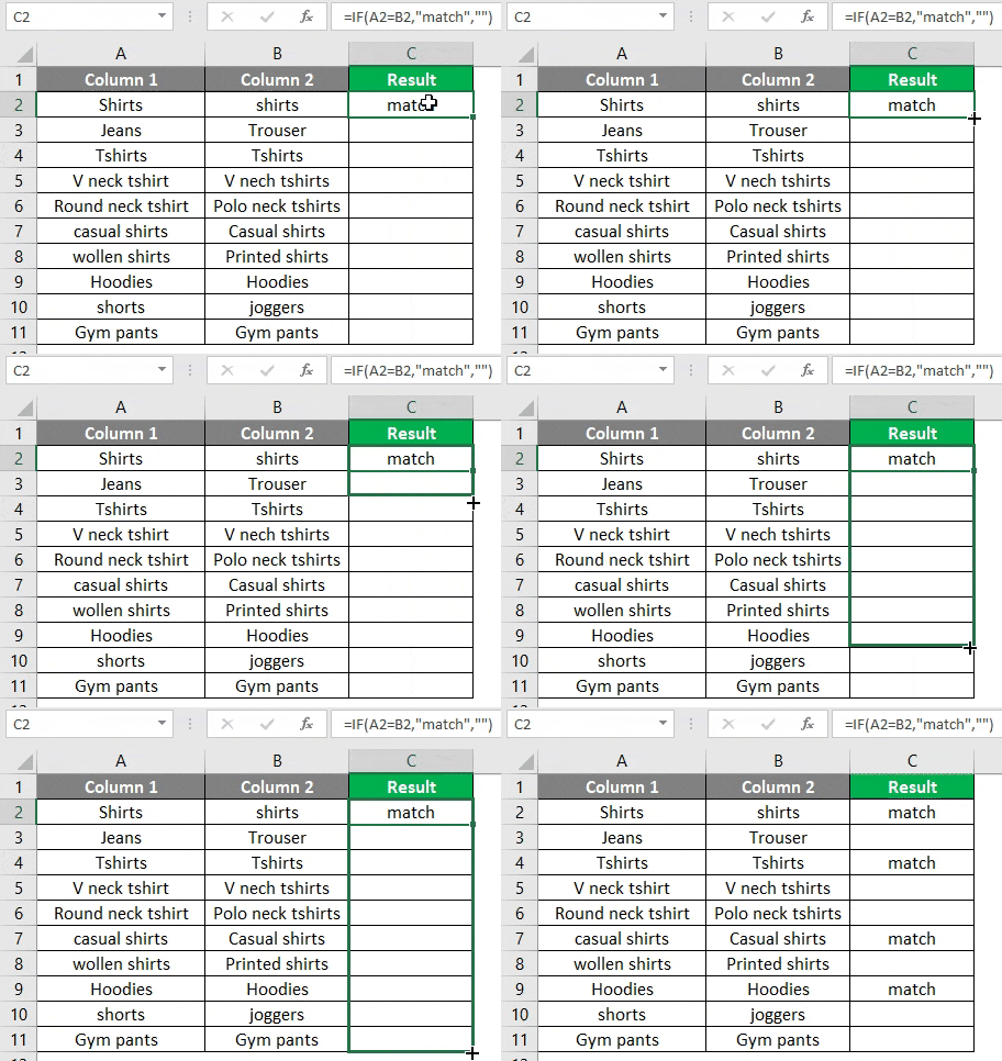
Drag the same formula in cell C2 to cell C11.
The matching cells yielded a result as a match, and the unmatched are indicated as blank.
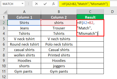
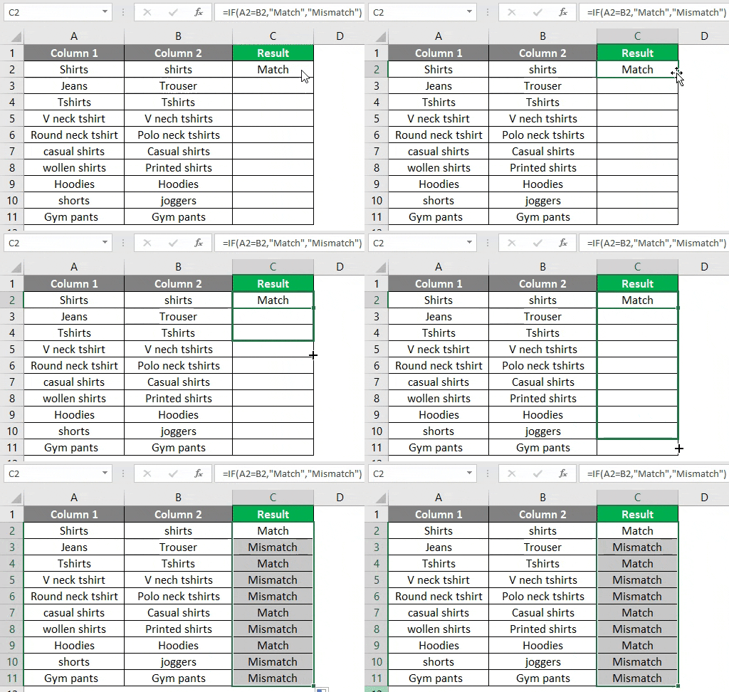
Another way to indicate cells can be done in the below manner. We will write the below formula in cell C2.
This will indicate the matching cells as “Match” and different cells as “Mismatch”.
We can also compare case sensitive data in two columns in the same row.
Example #3 – Finding the Case Sensitive Match
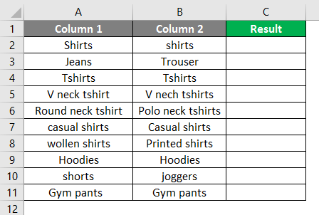
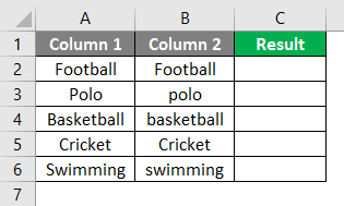
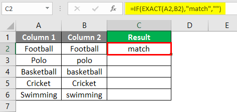
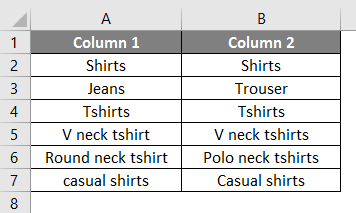
To go for a case sensitive match, we use the EXACT function. We have sample data to find case sensitive matches.
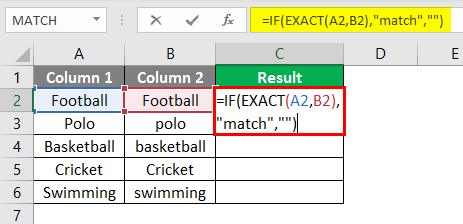
In cell C2, we will write the formula below.
After using the IF, the formula result is shown below.
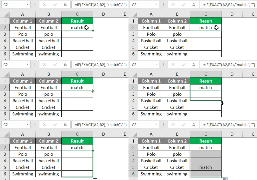
Drag the same formula in cell C2 to cell C6.
After writing the formula in cell c2, drag it downwards to see the case sensitive match of cells in the same row.
Highlighting Row Differences in Two Columns
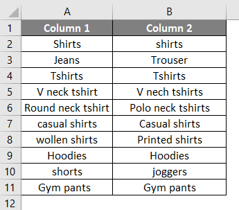
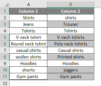
To highlight the cell in the second column that is different from the first in the below data table.
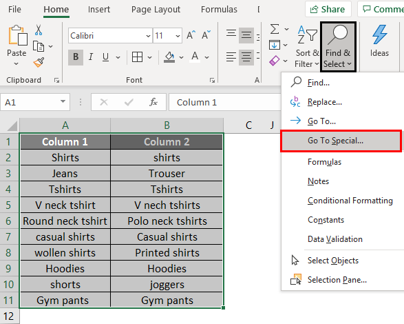
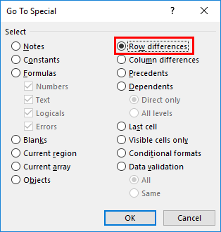
Select both columns, then go to the “Find & Select” tab and “Go to Special..”
Now select ‘Row differences.’
Press Enter Key. You will now see the unmatched cells highlighted.
Example #4 – Comparing More than 2 Different Columns
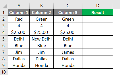
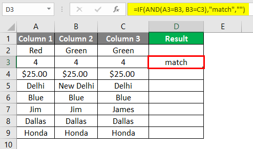
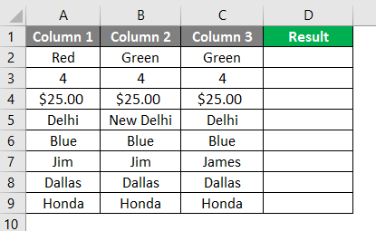
In this example, let’s compare more than 2 different columns for the match in the same row. In the below data table, we have to match all three columns in the same row and show the result in column D.
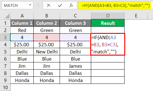
We will write the below formula in cell D3.
After using the formula, the result is shown below.
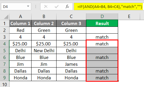
Drag the same formula into other cells.
We can see that columns A, B, and C have the same data in rows 3, 4,6,7, and 8, so the result is “match” while the data is different in other rows.
Example #5 – Finding Matching Cells in the Same Row
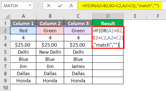
Now we will find the matching cells in the same row but only in 2 columns using the OR function.
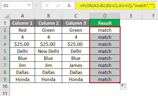
Taking our previous data table, we will write the below formula using the OR function in cell D2.
Press Enter, then drag it downwards.
We can see that any two columns with the same data match.
Example #6 – Compare Two Columns to Find Matches and Differences
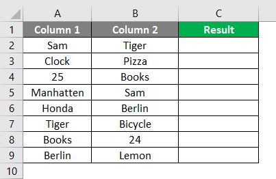
We have data in two columns and want to find all the text, strings, or numbers in column A but not in column B.
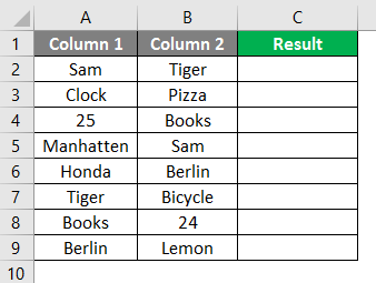
This way, we will compare the two columns and find the matching and different values. Below is sample data in which we will compare columns A and B to find the matching data.
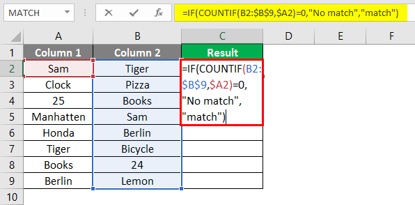
We will write this formula in cell C2 to get the desired result.
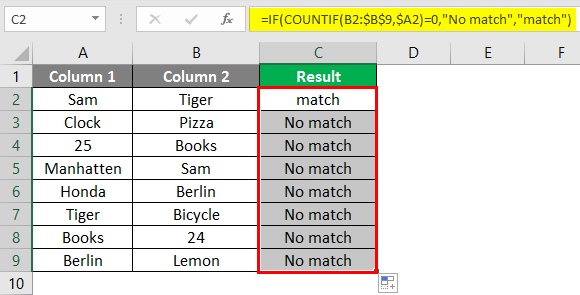
We will write the formula, press Enter, and then drag it downwards to see the result. In the below formula, we have used COUNTIF with IF. The COUNTIF formula searches A1, A2, and so on in column B, and IF gives it a condition that if there is 0, it will return “No match”; if the value returned by COUNTIF is 1, it will be a match.
In the above example, the COUNTIF function searched A1 in column B, A2 in column B, C1 in column B, and so on until it found the value in A and returned “match”.
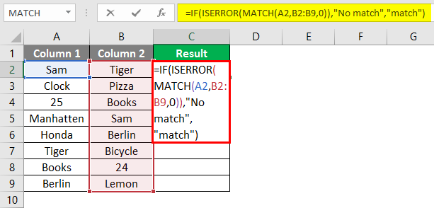
We can also get the same result by using the Match function.
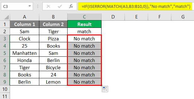
Now drag it downwards.
We get the same result with this formula as well.
Example #7 – Compare Two Columns and Highlight the Matches and Differences
We can compare and highlight column A entries found in Column B by using Conditional Formatting.
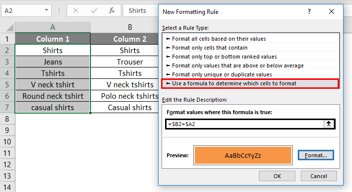
Select the column in which you want to highlight the cells. Then click the Conditional Formatting Tab and “use a formula to determine which cells to format“.
Click on OK.
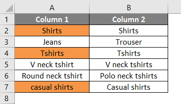
Cells that match in both columns are highlighted. In the same way, we can highlight the cells that are not matching.
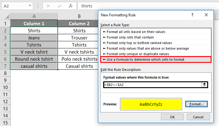
Select the column in which you want the cells different from being highlighted.
Now click on OK.
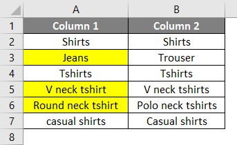
All the cells of column 1 that are not found in column 2 are highlighted.
The above examples are some of the ways to compare two columns. We can find the matches and differences in two or more columns through the above examples.
Things to Remember About Matching Columns in Excel
- We can compare the data in two or more columns in the same row.
- Both the columns should be of the same size.
- If any cells are left blank, the result will be blank.
- This is a case sensitive thing. The same data in different cases will lead to an unmatched result. The exact function is used to compare case sensitive data and get a correct result.
Recommended Articles
This is a guide to Matching Columns in Excel. Here we discuss How to use Matching Columns in Excel, practical examples, and a downloadable Excel template. You can also go through our other suggested articles –

