Updated March 4, 2023

Introduction to Matlab fft()
Matlab method fft() carries out the operation of finding Fast Fourier transform for any sequence or continuous signal. A FFT (Fast Fourier Transform) can be defined as an algorithm that can compute DFT (Discrete Fourier Transform) for a signal or a sequence or compute IDFT (Inverse DFT). Fourier analysis operation on any signal or sequence maps it from the original domain (usually space or time) to that of the frequency domain, whereas IDDFT carries out the reverse operation.
Syntax:
| Syntax | Description |
| F = fft(f) | This form of the command is to compute DFT (Discrete Fourier Transform) of ‘f’ using a FFT (Fast Fourier transform) algorithm and results the frequency domain signal F. |
| F = fft(f, n) | This form of the command is to compute DFT (Discrete Fourier Transform) of ‘f’ using a FFT (Fast Fourier Transform) algorithm and results the frequency domain n-point DFT signal ‘F’. BY default F possess same size as that of f. |
| F = fft(f, n, dim) | This form of the command is to compute DFT (Discrete Fourier Transform) of ‘f’ using a FFT (Fast Fourier Transform) algorithm and results the frequency domain FT signal ‘F’along the dimension ‘dim’. |
Examples of Matlab fft()
Given below are the examples mentioned:
Example #1
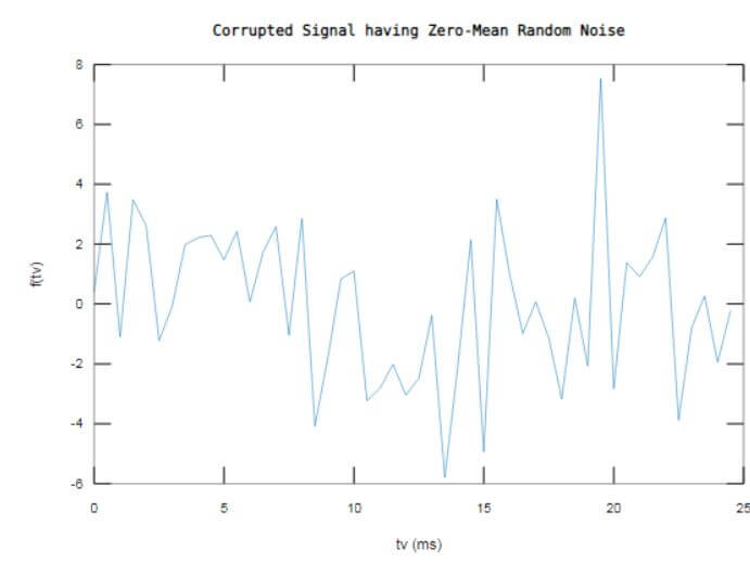
Deriving FFT for Random Noise Signal.
Code:
Ls = 2500;% Signal length

Fs = 2000;% Sampling frequency

Ts = 1/Fs;% Sampling period

tv = (0:Ls-1)*Ts;        % Time vector

f = 0.6*sin(2*pi*50*tv) + 3*randn(size(tv))+ sin(2*pi*120*tv);%Input signal

plot(1000*tv(1:50),f(1:50))

xlabel('tv (ms)')

ylabel('f(tv)')

title(' Corrupted Signal having Zero-Mean Random Noise')

F = fft(f);% Calling fft() function for signal ‘f’

PS2 = abs(F/Ls);% Double sampling plot

PS1 = PS2(1:Ls/2+1);% Single sampling plot

PS1(2:end-1) = 2*PS1(2:end-1);

f = Fs*(0:(Ls/2))/Ls;

plot(f,PS1)

title('Amplitude Spectrum (Single-Sided) PS1 for f(t)')

xlabel('f (Herz)')

ylabel('|PS1(f)|')
Output:
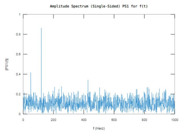
The output window displays the noise signal formed as function ‘f’ in time domain and single sided amplitude spectrum is computed using fft() resulting in frequency domain signal ‘F’.
The nature of the resultant FFT signal varies depending on the type of input signal or data such as:
| Nature of Input | Nature of Output |
| f is a Vector | F is produced as Fourier transform of vector f. |
| f is a Matrix | F is produced as Fourier transform of each column of matrix ‘f’. |
| f is a multidimensional array | Function fft(f) treats the values along the first non-unit array dimension as vectors and returns the Fourier transform for each vector. |
Example #2
Deriving np point FFT for Gaussian Signal.
Code:
Fs = 300;   % Sampling frequency

ts = -0.5:1/Fs:0.5;  % Time vector

Ls = length(ts);   % Signal length

f = 1/(4*sqrt(2*pi*0.02))*(exp(-ts.^2/(2*0.02)));

plot(ts,f)

xlabel('Time (t)')

ylabel('f(t)')

title('Time Domain')

np = 2^nextpow2(Ls);

f = Fs*(0:(np/2))/np;

F = fft(f,np);

PF = abs(F/np);

plot(f,PF(1:np/2+1))

xlabel('(f)')

ylabel('|PF(f)|')

title('Frequency Domain')
Output:
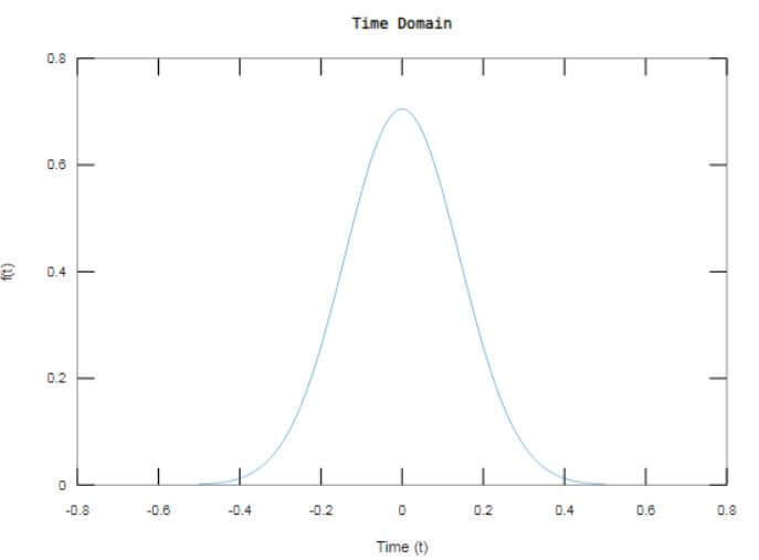
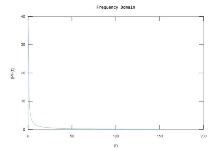
The output window displays the Gaussian signal formed as function ‘f’ in time domain and np-point FFT is computed using fft() resulting in frequency domain signal ‘PF’.
The nature of the resultant n-point FFT signal varies depending on the type of input signal or data such as:
| Nature of Input | Nature of Output |
| f is a Vector having length smaller than the value of ‘n’. | F is produced as Fourier transform of vector f being padded with trailing zeros to match the length of ‘n’. |
| f is a Vector having length greater than the value of ‘n’. | F is produced as Fourier transform of vector f being truncated to the length of ‘n’. |
| f is a matrix | F is produced as Fourier transform of each column of matrix ‘f’. |
| f is a multidimensional array | Function fft(f) treats the values along the first non-unit array dimension as vectors and returns the Fourier transform for each vector. |
Example #3
Code:
Fs = 2000;   % Sampling frequency

Ts = 1/Fs;   % Sampling period

Ls = 3000;   % Length of signal

t = (0:Ls-1)*Ts;        % Time vector

r1 = sin(3*pi*60*t);   % waveformed in First row

r2 = sin(3*pi*140*t);   % waveformedin Second row

r3 = sin(3*pi*350*t);   % waveformedin Third row

% Display of all 3 waves in time domain

f = [r1; r2; r3];

for k = 1:3

subplot(3,1,k)

plot(t(1:200),f(k,1:200))

title(['Row No ',num2str(k),' (Time Domain)'])

end

np = 2^nextpow2(Ls);% Defining n value for DFT operation

d = 2;

F = fft(f,np,d);% Calling fft() for the matrix f  having each wave as one row

PS2 = abs(F/Ls);

PS1 = PS2(:,1:np/2+1);

PS1(:,2:end-1) = 2*PS1(:,2:end-1);

% Computing FFT of all 3 waves and displayed in frequency domain

for k=1:3

subplot(3,1,k)

plot(0:(Fs/np):(Fs/2-Fs/np),PS1(k,1:np/2))

title(['Row No',num2str(k),'(Frequency Domain)'])

end
Output:
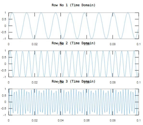
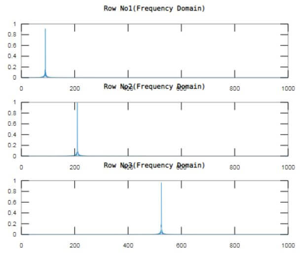
The output window displays the three sinusoidal waves r1, r2 an r3 in time domain and their respective single side amplitude spectrum is computed on the waves in the form of matrix f, using fft() resulting in frequency domain signal ‘PS1’.
How fft() works?
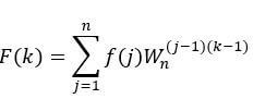
F = fft(f) calls the operation of Fourier transform whereas f = ifft(F) calls the operation of inverse Fourier transform. For f and F of length n, these transforms operations are defined as below:
Fourier transform F (frequency domain signal) for time or space domain signal f:
Inverse Fourier transform f (space or time domain signal) for signal F (frequency domain signal):
Where Wn is the nth root of the unity i.e.
Additional Note:
- fft() function execution time depends on the length defined for the transform to be carried out. The Transformation lengths with small prime factors are considerably faster than those with large prime factors.
- For most of the values of n, real-input DFTs get executed approximately within half the execution time of a complex-input DFTs.
- In case the value of n has large prime factors, the difference is speed is null or insignificant.
- The speed of fft() function can potentially be increased by implementing fftw, the utility function. This function, fftw can control the optimization of the algorithm used in the computation of an FFT operation performed with a particular size and dimension.
Recommended Articles
This is a guide to Matlab fft(). Here we discuss the introduction to Matlab fft(), how fft() works along with respective examples. You may also have a look at the following articles to learn more –
