Updated March 13, 2023

Definition of Matlab ksdensity Function
In Matlab ‘ks density’ function is used to calculate probability density function response. This function works on arrays, vectors, and multidimensional data. Probability density function uses normal kernel function to calculate density. By applying above function we get density values as well as density response curve of function. The evaluation of function is perform on equally spaced points on x time interval axis. It calculates density at hundred points and nine hundred points for uni- variants sample and bi variants sample respectively. Along with instance value it accepts other arguments also like name, value, axis, and points.
Syntax:
[A, B] = ksdensity (input);
Ksdensity (input, A, 'Function', 'icdf' )
Ksdensity (input variable name, variable name 1, ’function’, ‘ icdf ’)
[A, B, Bandwidth] = ksdensity (input)
How ksdensity function works in Matlab?
Density function has two different measures probability density function and cumulative density function. Probability density function can be achieved by integrating cumulative density function and cumulative density function can be achieved by differentiating probability density function. this function is used to interpret values at each given sample. we can pass multiple arguments through density function like density function, sample locations, bandwidth, input samples, CDF or pdf. to apply function initially we need to create input of continuous values or samples then only we can apply ksdensity function.
Examples
Let us discuss examples of Matlab ksdensity.
Example #1
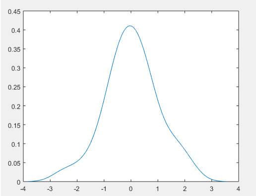
To apply ksdensity function first we need to create sample database, here we have created input sample data which is declared as ‘input’. Input is a combination of two normal random distribution. Random normal distribution is created by using randn function. first random function will give 25 by 1 matrix random values and second random function will give 10 by 1 matrix random value. this function will trace all the value in a range of input .here ‘A’ is probability density function and this function estimation is based on points ‘B’.
Code:
clc ;

clear all ;

disp ('output')

input = [randn(25, 1); randn(10, 1)];

[ A, B ] = ksdensity (input);

figure

plot (B, A);
Output :
Example #2
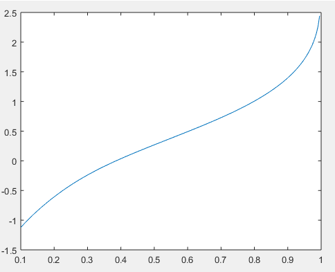
In this example, we will use another function inside ksdensity function. Initially, input samples are declared by the variable name ‘input’. Input is created by line space function which will create rows of vectors from 1 to 200. line space will create array or vector by pacing of sample 1.then we have used ksdensity function with multiple arguments we are passing input and A to the function. Input is created by combining two random functions; first random function will create samples in rage of fifty to 1 that means matrix of fifty by one and second random function will create random samples in range of ten to 1 that means matrix of ten by one. here ‘A’ is probability density function and this function estimation is based on points in input. Along with these two parameter other parameter pass through the function are ‘function and icdf’. Here function is keyword for ‘icdf’ and icdf is inverse cumulative distributed function which will perform inverse operation of cumulative distribution function.
Code:
clc ;

clear all ;

disp ('output')

input = [randn(50, 1); randn(10, 1)];

A = linspace(.1, 1, 200);

figure

ksdensity (input, A, 'Function', 'icdf');
Output:
Example #3
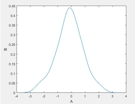
In this example, we will consider one more new term which is bandwidth. Bandwidth specifies how much sample rate passed through function. Here we have created input sample data which is declared as ‘input’. Input is a combination of two normal random distribution. Random normal distribution is created by using randn function. First random function will give fifteen by one matrix random value and second random function will give fifty by one matrix random value. this function will trace all the value in range of input .here ‘A’ is probability density function and this function estimation is based on points ‘B’. we are giving format of three variables to the function so automatically ksdensity function will return values of A, B, and Bandwidth.
Code:
clc ;

clear all ;

disp ('output')

input = [randn(15, 1) ; randn(50, 1)];

[ A, B, Bandwidth] = ksdensity (input);

Bandwidth

figure

plot (B, A);

xlabel ('A')

ylabel ('B')

hold on
Output:
Conclusion
In this article, we have seen ksdensity function implementation. It includes implementation of probability density function as well as the cumulative density function. This function gives density value at all the possible instances of a continuous signal as well as it gives curve response of function with respect to input signal.
Recommended Articles
This is a guide to Matlab ksdensity. Here we discuss the definition, How ksdensity function work in Matlab? and examples with code implementation respectively. You may also have a look at the following articles to learn more –


