Introduction to Matlab Root Finding
Roots of a polynomial are the values for which the polynomial equates to zero. So, if we have a polynomial in ‘x’, then the roots of this polynomial are the values that can be substituted in place of ‘x’ to make the polynomial equal to zero. Roots are also referred to as Zeros of the polynomial.
- If a polynomial has real roots, then the values of the roots are also the x-intercepts of the polynomial.
- If there are no real roots, the polynomial will not cut the x-axis at any point.
In MATLAB we use ‘roots’ function for finding the roots of a polynomial.
Syntax:
R = roots (Poly)
Description:
- R = roots (Poly) is used to find the roots of the input polynomial
- The input polynomial is passed as an argument in the form of a column vector
- For a polynomial of degree ‘p’, this column vector contains ‘p+1’ coefficients of the polynomial
Roots Function in Matlab with Examples
Let us now understand the code of roots functions in MATLAB using different examples:
Example #1
In this example, we will take a polynomial of degree 2. We will follow the following steps:
- Let our input polynomial be x^2 – x – 6
- Initialize the input polynomial in the form a column vector
- Passthiscolumn vector as an argument to the root function
Code:
Poly = [1 -1 -6]
R = roots(Poly)
Input:
Poly = [1 -1 -6];

R = roots(Poly)
Output:
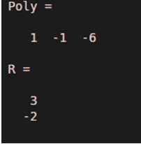
As we can see in the output, roots of the input polynomial x^2 – x -6 are 3, -2, which are the same as expected by us.
Example #2
In this example, we will take a polynomial of degree 3. We will follow the following steps:
- Let our input polynomial be x^3 –5x^2 + 2x+8
- Initialize the input polynomial in the form a column vector
- Pass this column vector as an argument to the root function
Code:
Poly = [1 -52 8]
R = roots(Poly)
Input:
Poly = [1 -5 2 8];

R = roots(Poly)
Output:
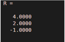
As we can see in the output, roots of the input polynomial x^3 – 5x^2 +2x +8 are 4, 2, -1, which are the same as expected by us.
Example #3
In the above 2 examples, we had polynomials with real roots. Let us now take some examples where polynomials have non-real roots.
In this example, we will take a polynomial of degree 5. We will follow the following steps:
- Let our input polynomial be x^5+2x^2 + x-2
- Initialize the input polynomial in the form a column vector
- Pass this column vector as an argument to the root function
Code:
Poly = [1 0 0 2 1 -2]
R = roots(Poly)
Input:
Poly = [1 0 0 2 1 -2]
R = roots(Poly)
Output:
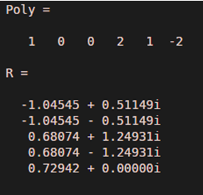
As we can see in the output, we have obtained complex roots for the input polynomial x^5 +2x^2 + x -2, as expected by us.
Example #4
In this example, we will take a polynomial of degree 2 and with complex roots. We will follow the following steps:
- Let our input polynomial be x^2 + 1
- Initialize the input polynomial in the form a column vector
- Pass this column vector as an argument to the root function
Code:
Poly = [1 0 1]
R = roots(Poly)
Input:
Poly = [1 0 1]
R = roots(Poly)
Output:
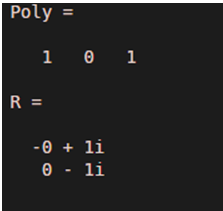
As we can see in the output, we have obtained complex roots for the input polynomial x^2 + 1, as expected by us.
Example #5
In this example, we will take a polynomial of degree 3 with real roots. We will follow the following steps:
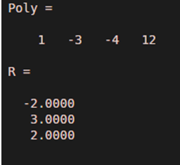
- Let our input polynomial be x^3 – 3x^2 – 4x + 12
- Initialize the input polynomial in the form a column vector
- Pass this column vector as an argument to the root function
Code:
Poly = [1-3-4 12]
R = roots(Poly)
Input:
Poly = [1 -3 -4 12]
R = roots(Poly)
Output:
As we can see in the output, the roots of the polynomial x^3 -3x^2 -4x 12 are -2, 3, 2
Recommended Articles
This is a guide to Matlab Root Finding. Here we also discuss the introduction and roots function in Matlab along with different examples and its code implementation. you may also have a look at the following articles to learn more –

