Updated February 28, 2023
Introduction to Matlab stem()
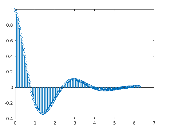
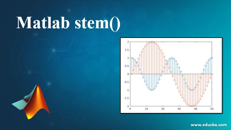
Stem() method in MATLAB is a type of plotting method to represent any type of data in a discrete form. This method generates a plot in the form of vertical lines being extended from the bases line, having little circles at tips which represents the exact value of the given data. Unlike plot() function, it does not join the values points with each other to create a continuous graph, rather it emphasizes the fact that the data points are discrete, not continuous.
Syntax:
There are various syntax that are available to implement stem() method based on a number of vectors and attributes, used as input argument.
Stem(Y)
Where Y is a data sequence to be presented in the plot.
Stem(X,Y)
Where X and Y are input vectors and the plot is generated for Y data points with respect to the X data point.
Stem(X,Y,a1,a1 value, a2, a2 value,…..,an ,an value)
Where X and Y are input vectors and an is the attribute name and an value is the value corresponding to an attribute.
Example:
figure

% Defining base line - X input vector ranging from 0 to 2*pi

X = 0 : pi/100 : 2*pi;

% Defining the Y input vector as function of X

Y = exp(-3*X/4) .* cos(2*X);

% Third, we use the 'stem' function to plot discrete values

stem(X,Y)
Output:
Properties of Stem()
MATLAB incorporates different attributes for stem() method that lets user to customize the appearance of the graph plot.
Some of those properties that are widely used are described in the table given below:
| Attribute | Description |
| Color | Decides the stem color. |
| ColorMode | Decides on how the color property is set-auto or manual. |
| LineStyle | Decides on the style to be adopted for stem line. |
| LineStyleMode | Decides on how the LineStyle property is set-auto or manual. |
| LineWidth | Used to control the width of the marker edge and the stem. |
| Marker | Decides the symbol to be used as a marker. |
| MarkerMode | Tells about how the marker property is filled. |
| MarkerSize | Defines the size of the marker. |
| MarkerEdgeColor | Decides on the color for the outline of the marker. |
| MarkerFaceColor | Decides on the color to fill in the marker. |
| BaseValue | Decides the value for baseline depending on the orientation of the plot. |
| BaseLineValue | Decides on the value to be displayed on the baseline. |
| ShowBaseLine | Set the visibility status of the baseline. |
| DisplayName | Sets the label for legend in the plot. |
| Annotation | Used to decide inclusion or exclusion of object from a legend. |
| Visible | Decides on the state of visibility for an object. |
| UIContextMenu | Sets the context menu to be displayed on right-click on the selected object |
| SelectionHighLight | Used to decide on displaying of selection handles when an object is selected. |
| Clipping | Used to restrict the object to the limits of the axes. |
| BusyAction | Decides on how MATLAB should handle the execution of interrupting callbacks. |
| PickableParts | Decides on permitting clicked part of the stem object by mouse, to be captured or not. |
| Tag | Used as an object identifier for a stem object. |
| UserData | Used to store arbitrary data over a stem object. |
| HandleVisibility | Decides on the visibility of the object handler. |
Examples of Matlab stem()
Following are the example are:
Example #1
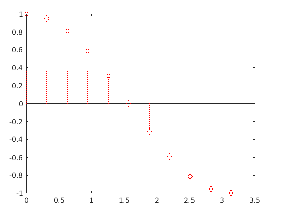
In the below program, stem() is used with setting the marker style diamond.
Code:
figure

X = 0 : pi/10 : pi;

Y = (cos(X));

stem(X,Y,':diamondr')
Output:
Example #2
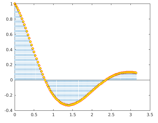
The below example demonstrates the change in the stem plot by using the attributes Linestyle, MarkerFaceColor, and MarkerEdgeColor:
Code:
figure

% Defining base line - X input vector ranging from 0 to 2*pi

X = 0 : pi/100 : pi;

% Defining the Y input vector as function of X

Y = exp(-3*X/4) .* cos(2*X);

% Syntax is used to set LineStyle as ‘-.’, Marker color as yellow and border of %the marker as red

stem(X,Y,'LineStyle','-.',...

'MarkerFaceColor','yellow',...

'MarkerEdgeColor','red')
Output:
Types of Plots Generated Using Stem()
Types of plots generated using stem() are given below:
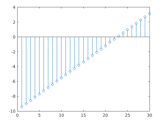
1. Plotting Single data series: The plot is generated for a single set of data points as shown in the below example:
Code:
figure

DATA = linspace(-3*pi,pi,30);

stem(DATA)
Output:
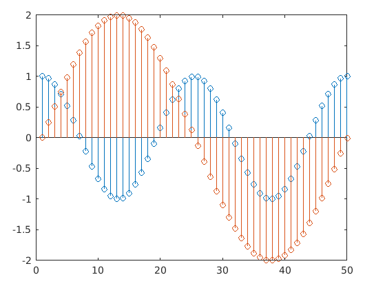
2. Plotting Multiple Data Series: Stem() method supports incorporating multiple sets of data points in one single plot as demonstrated in the below example:
Code:
figure

X = linspace(0,2*pi,50)';

% Defining 2 sets of data points as element of the vector DATA

DATA = [cos(2*X), 2*sin(X)];

stem(DATA)
Output:
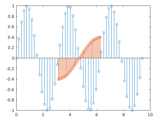
3. Plotting Multiple Data Series with Distinct Set of X-values: Stem() method has been adapted to extend its feature to present multiple sets of data points with respect to a different sets of X-values.
Code:
figure

% Defining 2 distinct sets of X-value points

xval1 = linspace(0,3*pi,50)';

xval2 = linspace(pi,2*pi,50)';

% Defining DATA1 baseline combining xval1 and xval2

DATA1 = [xval1, xval2];

% Defining 2 distinct sets of Y data points that are gives as element for DATA2

DATA2 = [sin(2*xval1), 0.4*cos(xval2)];

stem(DATA1,DATA2)
Output:
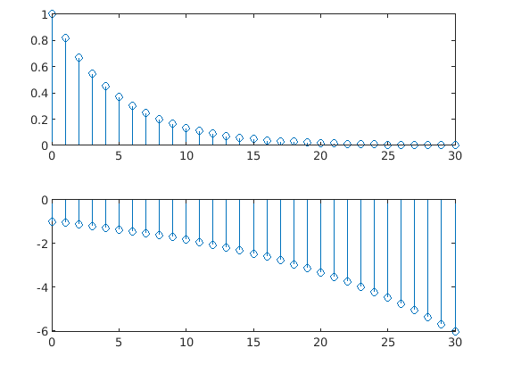
4. Plotting Multiple Data Series Stem within Single Layout: This feature enables the user to present multiple stem plots within one single layout.
Code:
xVAL = 0:30;

DATA1 = exp(-0.2*xVAL);

DATA2 = -exp(0.06*xVAL);

tiledlayout(2,1)

% Splitting the compete layout in 2X1 matrix

% Plotting the first stem graph in top segment

nt1 = nexttile;

% creating the axes object nt1

stem(nt1,xVAL,DATA1)

% Plotting the second stem graph in bottom segment

nt2 = nexttile;

% creating the axes object nt2

stem(nt2,xVAL,DATA2)
Output:
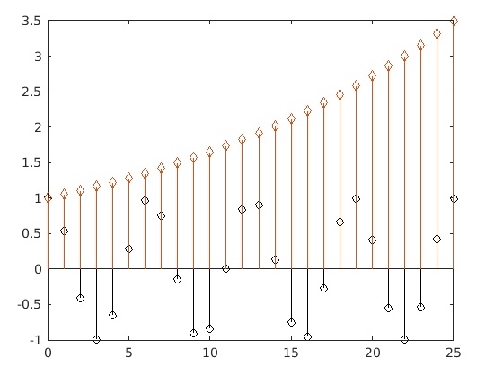
5. Customization of Plot After Creation: MATLAB has extended its feature for the stem method is to enable a user to customize the plot during a run time once the stem object is generated.
- Creation of Plot:
Xval = 0:25;

%Defining 2 different set of data points

DATA = [cos(Xval); exp(0.05*Xval)]';

%Defining h to store the stem object

h = stem(Xval,DATA);
- Customization of the Created Plot:
h(1).Color = 'black';

h(2).Marker = 'diamond';
Output:
Stem objects are considered to be unique identifiers. These allow a user to edit properties for a stem object during the run time after it is being created. It supports almost all common properties from MATLAB that are supported by a continuous plotting function plot(). In addition to those properties, it does have its own unique properties that provide a wide range of extensions to be applied to a discrete graph generated from the stem() method.
Recommended Articles
This is a guide to Matlab stem(). Here we discuss the Introduction and properties of stem() along with different examples and its code implementation. you may also have a look at the following articles to learn more –
