Introduction to Matlab trapz()
MATLAB has incorporated the function trapz to process numerical integration using trapezoidal rule-following unit spacing. This rule is defined to approximate a numerical integration for a definite time frame by dividing the area under the plot into tine sized trapezoids. It helps in forming easily computable areas. The function returns the single return value of type scalar which is the final value of the integration.
Preferably trapz is recommended to use for numerical integration on discrete type data sets.
Syntax
This integrating function trapz accepts different input arguments to decide on the behavior of the integration function, being used with different syntaxes respectively.
They are:
| Syntax | Description |
| Q = trapz(Y) | This syntax calculates the approximate integral value for ‘Y’ with unit spacing where the dimensions of the integration is determined based on the size of ‘Y’. |
| Q = trapz(X,Y) | This syntax calculates the approximate integral value for ‘Y’ with ‘X’ specified scalar spacing, where the dimensions of the integration is determined based on the size of ‘Y’. |
| Q = trapz(___,dim) | This syntax calculates the approximate integral value for the input with the dimensions of the integration given as ‘dim’. |
The input arguments that contribute to different syntaxes of the function trapz can be explained as below:
| Numeric Data-Y |
1. Y as vector àThe output is an approximated integral result for ‘Y’ 2. Y as matrixàThe output is the result of integration operation executed on each column, presented as a row vector of values of the integration operations. 3. Y as multi-dimensional arrayà The operation takes place on the first non-unit sized dimension of ‘Y’ and results in the size of value 1 for that dimension while the size of the other dimensions remains unchanged.
single/ double/ complex number |
| Point spacing-X |
1. X as vector à The length of the coordinate vector must be equal to the size of the first non-unit sized dimension of the numerical input ‘Y’. 2. X as scalaràIt satisfies the condition as trapz(Y, X) = X*trapz(Y)
|
| Dimensions for operation-dim |
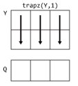
1. trapz(Y,1): It operates on elements with columns of ‘Y’, returning a row vector as output. 2. trapz(Y,2): It operates on elements with rows of ‘Y’, returning a column vector as output.
|
Examples of Matlab trapz()
Here are the following examples mention below:
Example #1 – Numerical integration with Unit spacing
This operation can be executed by applying the syntax Q = trapz(Y) in the trapz function implementation in the MATLAB code.
Code:
The below code snippet is written to execute trapz operation on input numeric ‘Y’ as f(x)= 10*2^x.
Y = [10 20 40 80 160 320];

Q = trapz(Y)
Output:
Example #2 – Numerical integration with Non-Unit spacing
This operation can be executed by applying the syntax Q = trapz(Y, X) in the trapz function implementation in the MATLAB code.
Code:
The below code is written to call trapz function on input numeric data ‘Y’ having point spacing value of pi/10.
X = 0: pi/10:2*pi;

Y = cos(X);

Q = trapz(X,Y)
Output:
Example #3 – Numerical integration with non-uniform spacing
This operation can be executed by applying the syntax Q = trapz(Y, X, dim) in the trapz function implementation in the MATLAB code.
Code:
The below code is written to call the trapz function on the input numeric data ‘Y’ with non-uniform point spacing values defined by ‘X’ with the value of ‘dim’ as ‘2’.
The point spacing is obtained by matrix ‘X’ which indicates that the trapezoids are formed non-uniformly.
The rows in input numeric data ‘Y’ is obtained from velocity data taken at 3 different trials.
X = [1 3.5 5 10];

Y = [15.2   27.7   19.6   13.2;

24.8   17.0  20.5   24.5;

14.9   26.5  10.2   13.8];

Q = trapz(X,Y,2)
Output:
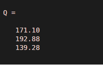
Trapz is executed on each row of the input numeric ‘Y’ as the value for ‘dim’ is set to 2. The resultant output is a column vector having an integration result for each row.
Example #4 – Multiple numerical integrations
The integration function trapz can also be used to perform double integral i.e integration in the format:
In order to perform trapz function on double integral expression, the function is called in the nested loop as demonstrated in the below example:
Code:
p = -5:.1:5;

q = -3:.1:3;

[P,Q] = meshgrid(p,q);

F = P.^2 + Q.^2;

I = trapz(q,trapz(p,F,2))
Output:
Example #5 – Real-time application of trapz
The trapz in MATLAB plays a vital role in integration calculations applied in real-time applications.
Code:
Trapz can be used to compute the average energy exhibited by an electrical machine for which v-i nonlinear relation is designed as:
The instantaneous voltage v(t)= sin(3t).
In the below code snippet the point spacing is defined by ‘time’ which is non-unit uniform spacing with the value of ‘10’.
The instantaneous power is calculated as p = f(i,v) = v*i.
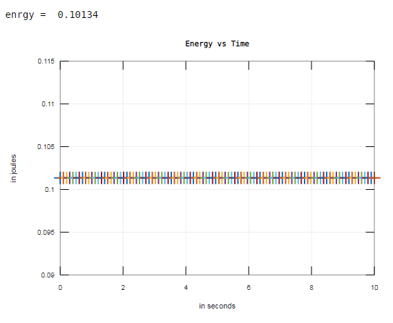
The average energy (enrgy) is calculated by applying the trapz function.
time=linspace (0,10,100);

volt=sin (3. *time); i=0.1*(exp (0.2.*volt)-1); p=volt.*i;

enrgy=trapz (time, p), plot (time, enrgy, '+'); grid; title ('Energy vs Time'); ...

xlabel('in seconds'); ylabel('in joules')
Output:
Additional Note
- The integration function trapz is similar to cumtrapz and difference lies as it reduces the dimension size to one and returns a single value without returning any intermediate values of integration.
- If input numeric data ‘Y’ is multidimensional array by nature, it works across the first non-singleton dimension whereas the size of other dimensions remains unaffected.
- It is similar to integral() and differs in the supported input data types. The function trapz works with discrete values whereas integral() works strictly with function (expression) integration operation.
Recommended Articles
This is a guide to Matlab trapz(). Here we discuss the different an introduction to Matlab trapz() with appropriate syntax and examples. You may also have a look at the following articles to learn more –


