Updated April 4, 2023

Definition of Mean Shift Clustering Python
Mean shift clustering in python is defined as a type of unsupervised learning algorithm in the field of data science that deals with grouping data points in a sample space. Unsupervised learning that class of machine learning algorithm that deals with identifying patterns in the data that doesn’t have any label attached to itself. And as the name suggests, that without any supervision, the algorithm is able to identify the patterns. The gist of the algorithm is to keep iteratively assign data points by moving the points towards the mode. Mode is the portion in the discrete data distribution where the density of the data point in the region is maximum and is typically the point of maxima. This algorithm is a non-parametric technique that is used for analysis and identification of the mode or maxima and is often referred to as mode-seeking algorithm.
Syntax
Importing the meanshift library in Python:
from sklearn.cluster import MeanShiftImporting the estimate bandwidth:
from sklearn.cluster import estimate_bandwidthThis library helps in determining the bandwidth which is used in a Radial Basis Kernel. This is calculated on the basis of average distances between the points that are in the cluster and is calculated pairwise.
Instantiating the object of the meanshift module that is imported:
<variable name> = MeanShift(bandwidth=None, seeds=None, bin_seeding=False, min_bin_freq=1, cluster_all=True, n_jobs=None, max_iter=300)The explanation of the different parameters is:
- bandwidth: Calculated for RBF kernel as explained in the above syntax.
- seeds: This parameter is to initialize the kernels. In case this is not set, by default seeds are calculated using clustering.get_bin_seeds and the bandwidth is used as the grid size.
- bin_seeding: This is a Boolean parameter, where when true, the initial kernel location is the location of discretized version of binned points and coarseness depends on the bandwidth.
- min_bin_freq: This parameter is set to accept only those bins that have a minimum seed as provided in this parameter
- cluster_all: This is a Boolean parameter as well and when true it makes sure that all the data points are clustered. In case of any outlier (ones with no clusters), they are assigned with the nearest cluster. On the other hand, when the argument is set to false the outliers are assigned -1 as a label
- n_jobs: This parameter is to denote the umber of jobs that is to be used for computation.
- max_iter: This denotes the maximum iterations that will take place before the job terminates until and unless the job hasn’t converged till then.
Fit the object variable of meanshift module that is declared:
<variable name>.fit(<data set>)How does Mean shift clustering works in python?
Firstly, let us get an intuition of the algorithm before jumping full-fledged into the core working. The intuition behind the working of mean shift clustering is on the lines of hierarchical clustering, where in initially each of the data points are assigned its own clusters. From then on, with a specified parameter the cluster groups different data point at each iteration until the group stops including any other data point. And with that, we get the clusters.
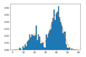
Now, going into a bit more depth, mean-shift algorithm builds on the concept of Kernel Density Estimate or KDE as an acronym. KDE is a method for estimating the underlying distribution of a dataset. In this method, a kernel is placed on each of the data points. For those who are not familiar with the concept of kernel, it is a simple weighing function that is used on the lines of any image processing to highlight or suppress a pixel value (depending on the use case). All these kernels when added together in a hierarchical fashion finally generates the probability distribution.
In the above graph, initially, all the histograms are a distribution and when the distribution of the neighbors are added, to reach to a higher peak than where it was previously till we see that there are no more peaks and in this way the plot in the above distribution, when there were no higher peaks near the 30-range, we don’t sum up the local maxima peak with the other maxima, and hence get the 2 maxima peaks!
In the same way, while executing mean shift in data distribution, all the data points are given distribution of its own. From now the chronological steps happen in order to get to the final clusters.
1. We take one single data point and perform the next steps. These steps are performed on all the data points in the space.
2. Using a bandwidth (a parameter we discussed in our syntax section), we draw a region around the data point and take all those points that are falling within that region.
3. Once we have lot of other data points, we find the mean of all those data points and assign the mean of those data points to be the new mean (This is where we do the mean shift).
4. The above process is repeated until the cluster no longer includes extra data point within it.
5. Once the process is repeated for all data points, we finally reach the clustered data points as if all the points in the sample space reach its corresponding local maximas.
Examples
Let us discuss an example of Mean Shift Clustering Python.
Mean shift clustering using sklearn module:
Code:
import numpy as np
import pandas as pd
from sklearn.cluster import MeanShift,estimate_bandwidth
from sklearn.datasets import make_blobs
from matplotlib import pyplot as plt
from mpl_toolkits.mplot3d import Axes3D
%matplotlib inline

clusters = [[27, 72, 91], [36, 90, 99], [9, 81, 99]]

#Making the random data set
X, _ = make_blobs(n_samples = 180, centers = clusters,
                                   cluster_std = 2.79)

# Estimating the bandwith (or the radius which needs to be taken as part of step 2)
bandwidth = estimate_bandwidth(X, quantile=0.2, n_samples=500)
meanshift = MeanShift(bandwidth=bandwidth)
meanshift.fit(X)
labels = meanshift.labels_
labels_unique = np.unique(labels)
n_clusters_ = len(labels_unique)

print('Estimated number of clusters: ' + str(n_clusters_))

y_pred  = meanshift.predict(X)
plt.scatter(X[:, 0], X[:, 1], c=y_pred, cmap="viridis")
plt.xlabel("Feature 1")
plt.ylabel("Feature 2")
Output:
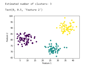
Here, we observe that there are 3 local minima that is possible with the random data set that is generated, and the data points are perfectly clustered in all the 3 points!
Conclusion
With the help of this article, we have got a glimpse of the mean shift clustering and also the module that enables the mean shift clustering. It is recommended to try out the basic mean shift clustering as part of practice without using the module so that we get the sense of algorithm (though it need not be fully optimized).
Recommended Articles
This is a guide to Mean Shift Clustering Python. Here we discuss the introduction, syntax, and working of Mean shift clustering in python along with an example and code implementation. You may also have a look at the following articles to learn more –


