Updated March 21, 2023
One–Way Analysis of Variance
A statistical concept, i.e. One Way ANOVA in R, proves useful when comparing means of a particular metric across various groups and specifically helps in analysis of only factor or variable, with certain assumptions related to the normal distribution of populations, equality of variance or standard deviation, and random and independent nature of samples, that must be followed as a pre-requisite, with R programming providing a very robust and effective set of methodologies for the implementation of the concept is referred to as.
Assumptions of Analysis of Variance
The following are the assumptions that must be met for applying one-way ANOVA:
- The populations from which the samples are drawn are normally distributed.
- The populations from which the samples are drawn have the same variance or standard deviation.
- The samples drawn from different populations are random and independent.
How One-Way ANOVA in R works?
For our demonstration, we are using the data which contains two variables viz: brand and Sales. There are four brands – ATB, JKV, MKL, and PRQ. Monthly sales for these brands are given. We need to check if mean sales across the four brands are equal or if they are different from each other. To verify this, we will use the One-way ANOVA. The step-by-step procedure to implement ANOVA is as follows:
1. First, import the data into R. The data is present in a CSV format. So, to import it, we will use the read.csv() function.
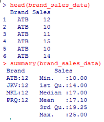
2. View the first few records of the data. This is important to check if the data has been rightly imported into R. Similarly, we will apply a summary() function over the data to get basic insights into the data.
3. Every time we use the dataset variables, we need to mention the dataset’s name like brand_sales_data$Brand or brand_sales_data$Sales explicitly. To overcome this, we shall employ the attach function. The function has to be applied as below.
4. Let’s aggregate Sales by Brand using mean or standard deviation. Aggregation helps us get a basic idea of data.
The above result shows means for the four different groups are not equal. JKV has the highest mean sales.
As shown above, the standard deviations across the four groups don’t show any significant difference, and it is highest for the brand MKL.
5. Now, we will apply ANOVA to validate if the means across the three populations are equal or there exists any difference.
From the results above, we can see that the ANOVA test for Brand is significant because of p < 0.0001. We can interpret that all brands don’t have the same preference levels in the market, which influences these brands’ sale in the market. This could be due to many factors and liking of people for a particular brand.
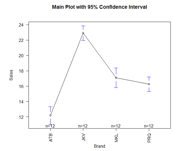
6. The above result can be visualized, and it makes interpretation easy. For that, we will use plotmeans() function in gplots() library. It works as below:
As we can see above, the plotmeans() function in the gplots package enables us to visually compare different groups’ means. We can see that means are not the same across the four brands. However, the means for the brands MKL and PRQ fall in close range.
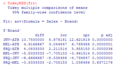
7. The above analysis helps us to check if brands have equal means or not; however, making the pair-wise comparison is difficult. We can make pair-wise comparisons for different brands using the TukeyHSD() function, which facilitates checking if a brand is significantly different from any remaining ones.
The pairwise comparisons as above. The difference between any two groups is significant if p < 0.001. As we can see above p-value for the PRQ-MKL pair is much higher, which indicates that the two brands aren’t significantly different from each other.
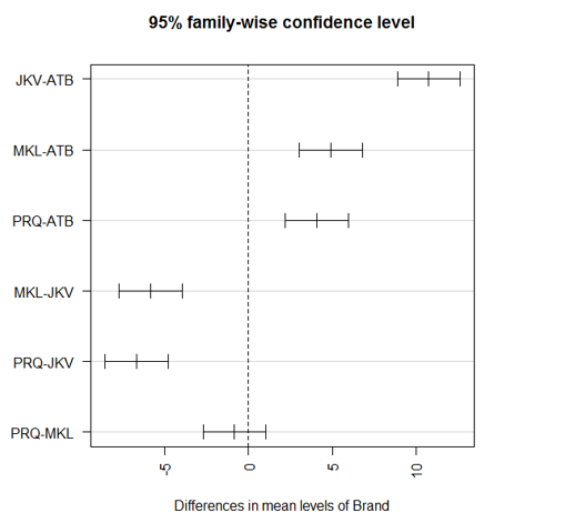
To visualize the pairwise comparisons, we will plot the above results as below:
The first par function rotates the axis labels making them horizontal, and the second par statement adjusts the margins so that the labels fit properly. Otherwise, they will go out of the screen.
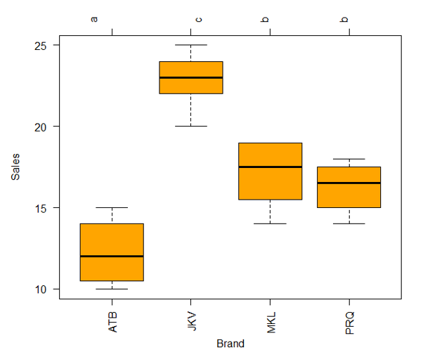
The above graph offers good insight, but we can plot the results in a boxplot to get better insights for clearer interpretation, as demonstrated below.
The glht() function used above comes with a comprehensive set of methods for comparing multiple means. Note, the level option in cld() function pertains to the significance level, e.g. 0.05 or 95 percent confidence)
Using the above plot, it becomes easy to compare means across the groups and facilitate systematic interpretation. There are letters, over the top of the plot, for each brand. If two brands have the same letter, they don’t have significantly different means as brands MKL and PRQ, which have the same letter b.
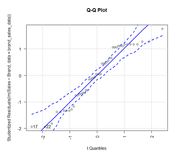
8. Till now, we implemented ANOVA and used plots to visualize the results. However, it is equally important to test the assumptions. First, we will validate the normality assumption.
The car package in R provides the function qqPlot(). The above plot shows that data falls within 95% confidence envelop. This indicates that the normality assumption has almost been met.
Next, we will validate if the variances across the brands are equal. For this, we will use Bartlett’s test.
The p-value shows that variances across the group don’t differ significantly.
Last but not least, we shall check if any outliers are there that affect ANOVA results.
From the above result, we can see that there’s no indication of outliers in the data (NA occurs when p > 1)
Considering the results of the QQ Plot, Bartlett’s test and Outlier test, we can say that data meets all ANOVA assumptions, and the results obtained are valid.
Conclusion – One Way ANOVA in R
ANOVA is a convenient statistical technique that can be used to compare means across multiple populations. R offers a comprehensive range of packages to implement ANOVA, derive results and validate the assumptions. In R, statistical results can be interpreted in visual forms that offer deeper insights.
Recommended Articles
This is a guide to One Way ANOVA in R. Here, we discuss How One-Way ANOVA works and the Assumptions of Analysis of Variance. You may also have a look at the following articles to learn more –
