Updated April 7, 2023

Introduction to OpenCV Optical Flow
The following article provides an outline for OpenCV Optical Flow. The pattern in which an image object moves from one frame to the consecutive frame due to the movement of the camera or due to the movement of the object is called optical flow and optical flow is represented by a two dimensional vector which is a displacement vector from one frame to the consecutive frame and the working of optical flow is based on two assumptions namely the intensities of the pixels in an image object do not change between the two consecutive frames and the motion of the neighboring pixels are same and we make use of two functions goodFeaturesToTrack() and calcOpticalFlowPyrLK() to implement optical flow.
Syntax to define calcOpticalFlowPyrLK() function in OpenCV:
calcOpticalFlowPyrLK(first_image, second_image, first_image_points, window_size, pyramid_level_number, criteria)Where,
- first_image is the first input image.
- second_image is the second input image.
- first_image_points are the feature points detected in the first image using goodFeaturesToTrack() function.
- window_size represents the integration window size.
- pyramid_level_number represents the pyramids allowing us to find optical flow ate different resolutions of the image. If this value is set to 0, no pyramids are used, if this value is set to 1, two pyramids are used and so on.
Working of calcOpticalFlowPyrLK() Function in OpenCV
- The pattern of the motion of the image object from one frame to the consecutive due to camera’s movement or object’s movement is called optical flow.
- The optical flow is represented by two dimensional vector also called as displacement vector.
- The optical flow can be found out by implementing the Lucas Kanade algorithm.
- The working of optical flow based on Lucas Kanade algorithm begins by finding the feature points in the input video.
- We make use of a function called goodFeaturesToTrack() function to track the feature points in the input video.
- The feature points detected using goodFeaturesToTrack() function will be tracked as displacement vectors by implementing the Lucas Kanade algorithm using calcOpticalFlowPyrLK() function.
- The calcOpticalFlowPyrLK() function returns an image consisting of two dimensional output vector points representing the optical flow.
Examples of OpenCV Optical Flow
Given below are the examples of OpenCV Optical Flow:
Example #1
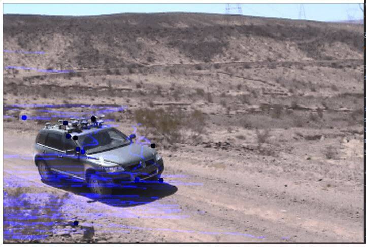
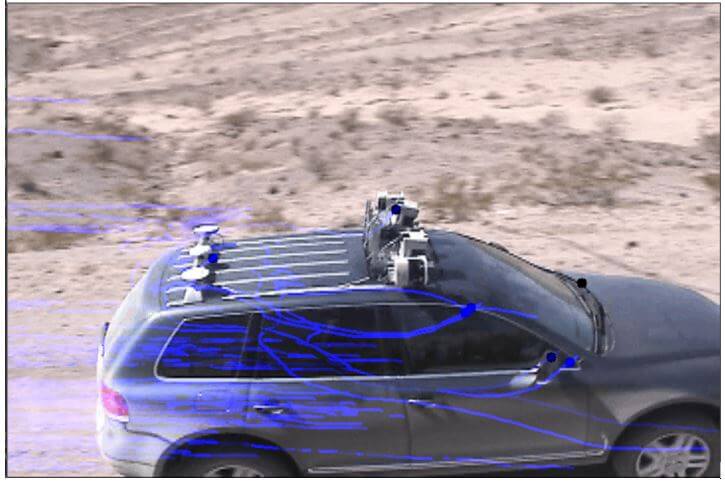
OpenCV program in python to demonstrate calcOpticalFlowPyrLK() function to determine the optical flow based on Lucas Kanade algorithm for the given input video and display the output on the screen.
Code:
#importing the required modules
import numpy as np
import cv2
#reading the input video whose optical flow is to be determined
videoread = cv2.VideoCapture("C:/Users/admin/Desktop/images/optical_flow_input.avi")
#defining the parameters to pass to the goodFeaturesToTrack() function as a dictionary
feature_points = dict(maxCorners=100,
qualityLevel=0.3,
minDistance=7,
blockSize=7)
#defining the parameters to pass to the calcOpticalFlowPyrLK() function as a dictionary
parameters = dict(winSize=(15, 15),
maxLevel=2,
criteria=(cv2.TERM_CRITERIA_EPS | cv2.TERM_CRITERIA_COUNT,
10, 0.03))
#generating random colors to apply to the resulting 2D vectors
resultingvectorcolor = np.random.randint(0, 255, (100, 3))
#finding the feature points in the first frame using goodFeaturesToTrack() function
first, first_frame = videoread.read()
first_gray = cv2.cvtColor(first_frame,
cv2.COLOR_BGR2GRAY)
points = cv2.goodFeaturesToTrack(first_gray, mask=None,
**feature_points)
#mask image is created for drawing the vectors
resmask = np.zeros_like(first_frame)
while (1):
second, second_frame = videoread.read()
second_gray = cv2.cvtColor(second_frame,
cv2.COLOR_BGR2GRAY)
#optical flow is calculated using calcOpticalFlowPyrLK() function
respoints, status, errors = cv2.calcOpticalFlowPyrLK(first_gray,
second_gray,
points, None,
**parameters)
#choosing the good points
good_second = respoints[status == 1]
good_first = points[status == 1]
#drawing the tracks
for i, (first, second) in enumerate(zip(good_second,
good_first)):
A, B = second.ravel()
C, D = first.ravel()
resmask = cv2.line(resmask, (A, B), (C, D),
resultingvectorcolor[i].tolist(), 2)
second_frame = cv2.circle(second_frame, (A, B), 5,
resultingvectorcolor[i].tolist(), -1)
resvideo = cv2.add(second_frame, resmask)
cv2.imshow('Result', resvideo)
k = cv2.waitKey(25)
if k == 27:
break
#the previous frame and points are updated
first_gray = second_gray.copy()
points = good_second.reshape(-1, 1, 2)
cv2.destroyAllWindows()
videoread.release()
Output:
In the above program, we are importing the required modules. Then we are reading the reading the input video whose optical flow is to be determined. Then we are defining the parameters to pass to the goodFeaturesToTrack() function as a dictionary. Then we are. Then we are generating random colors to apply to the resulting 2D vectors. Then we are finding the feature points in the first frame using goodFeaturesToTrack() function. Then a mask image is created for drawing the vectors. Then optical flow is calculated using calcOpticalFlowPyrLK() function. Then good points are chosen to draw the tracks. Then the previous frame and previous points are updated.
Example #2
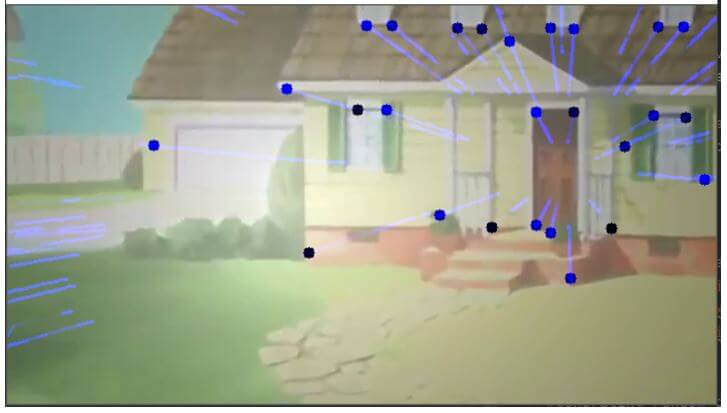
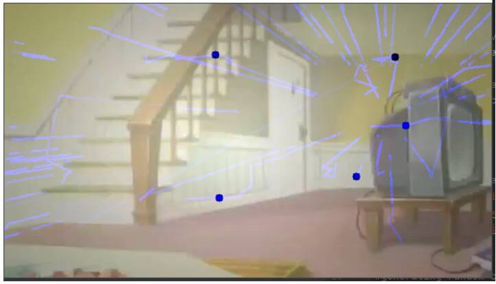
OpenCV program in python to demonstrate calcOpticalFlowPyrLK() function to determine the optical flow based on Lucas Kanade algorithm for the given input video and display the output on the screen.
Code:
#importing the required modules
import numpy as np
import cv2
#reading the input video whose optical flow is to be determined
videoread = cv2.VideoCapture("C:/Users/admin/Desktop/images/Tom and jerry.mp4")
#defining the parameters to pass to the goodFeaturesToTrack() function as a dictionary
feature_points = dict(maxCorners=100,
qualityLevel=0.3,
minDistance=7,
blockSize=7)
#defining the parameters to pass to the calcOpticalFlowPyrLK() function as a dictionary
parameters = dict(winSize=(15, 15),
maxLevel=2,
criteria=(cv2.TERM_CRITERIA_EPS | cv2.TERM_CRITERIA_COUNT,
10, 0.03))
#generating random colors to apply to the resulting 2D vectors
resultingvectorcolor = np.random.randint(0, 255, (100, 3))
#finding the feature points in the first frame using goodFeaturesToTrack() function
first, first_frame = videoread.read()
first_gray = cv2.cvtColor(first_frame,
cv2.COLOR_BGR2GRAY)
points = cv2.goodFeaturesToTrack(first_gray, mask=None,
**feature_points)
#mask image is created for drawing the vectors
resmask = np.zeros_like(first_frame)
while (1):
second, second_frame = videoread.read()
second_gray = cv2.cvtColor(second_frame,
cv2.COLOR_BGR2GRAY)
#optical flow is calculated using calcOpticalFlowPyrLK() function
respoints, status, errors = cv2.calcOpticalFlowPyrLK(first_gray,
second_gray,
points, None,
**parameters)
#choosing the good points
good_second = respoints[status == 1]
good_first = points[status == 1]
#drawing the tracks
for i, (first, second) in enumerate(zip(good_second,
good_first)):
A, B = second.ravel()
C, D = first.ravel()
resmask = cv2.line(resmask, (A, B), (C, D),
resultingvectorcolor[i].tolist(), 2)
second_frame = cv2.circle(second_frame, (A, B), 5,
resultingvectorcolor[i].tolist(), -1)
resvideo = cv2.add(second_frame, resmask)
cv2.imshow('Result', resvideo)
k = cv2.waitKey(25)
if k == 27:
break
#the previous frame and points are updated
first_gray = second_gray.copy()
points = good_second.reshape(-1, 1, 2)
cv2.destroyAllWindows()
videoread.release()
Output:
In the above program, we are importing the required modules. Then we are reading the reading the input video whose optical flow is to be determined. Then we are defining the parameters to pass to the goodFeaturesToTrack() function as a dictionary. Then we are. Then we are generating random colors to apply to the resulting 2D vectors. Then we are finding the feature points in the first frame using goodFeaturesToTrack() function. Then a mask image is created for drawing the vectors. Then optical flow is calculated using calcOpticalFlowPyrLK() function. Then good points are chosen to draw the tracks. Then the previous frame and previous points are updated.
Conclusion
In this article, we have seen the concept of optical flow based on Lucas kanade algorithm with corresponding programming examples and their outputs to demonstrate them.
Recommended Articles
We hope that this EDUCBA information on “OpenCV Optical Flow” was beneficial to you. You can view EDUCBA’s recommended articles for more information.


