Updated August 16, 2023
Introduction to Opposite of Concatenate in Excel
As we all know, the Excel Concatenate function can combine multiple strings in one cell. However, in some situations, you might need to do the opposite of concatenating, i.e., split the combined text into different columns. In such situations, what can we do? We have solutions for such cases. We can use Excel’s Text to Column feature and Flash Fill option. We can also use some custom formulae to split the concatenated text. Let’s see the methods one by one.
How to Use Opposite of Concatenate in Excel?
Excel Concatenate function is very simple and easy. Let’s understand how to use this function in Excel with some examples.
Example #1 – Split cells using Text to Column
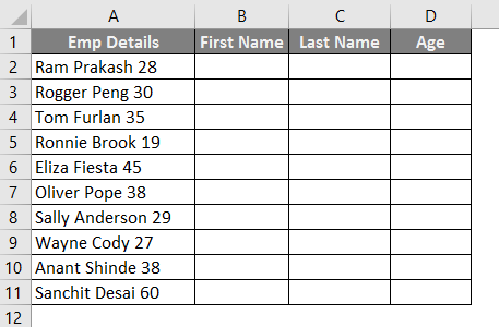
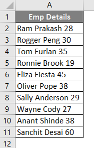
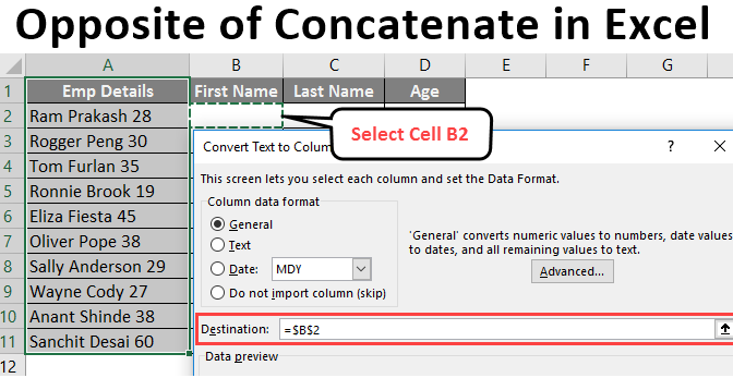
We can split texts with different methods and different formulae. However, one of the simplest, best, and most time-saving methods in Excel’s Text to column facility is to split the text into different columns. Suppose we have data as below, and we wanted the information of Employee’s Name and Age in two columns named B and C.
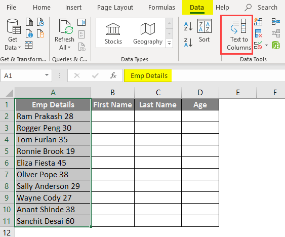
- Go to Data in the uppermost pane and select Text to Column wizard in Excel.
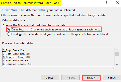
- Once you click Text to Column Wizard, a new window named Convert Text to Columns Wizard will pop up. Here select the Delimited option to separate the text. Click Next.
- Click Next> and you’ll see a preview of the split text. Excel takes a guess where the split should be in the data.
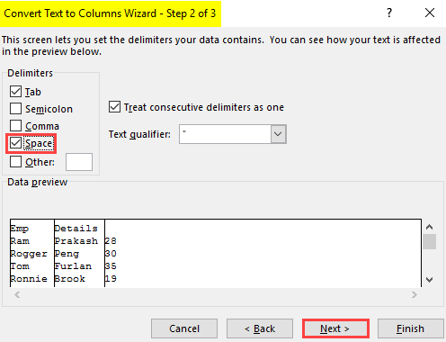
In this case, Excel guessed that the spill should happen wherever there is a space. Therefore it checked the box of Space under Delimiters and showed Data Preview as in the image above.
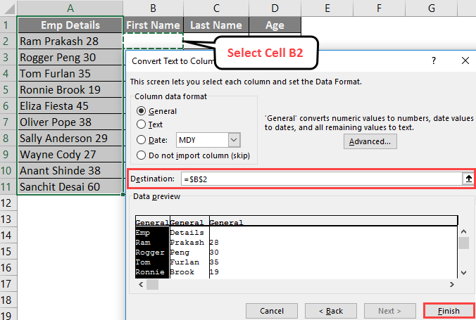
- Click Next> You’ll be popped up to the screen where you can now select the Data Format for each column and set the Destination for the split to be done at.
You can change the format of each split preview by simply clicking on the radio button next to the different Column data formats. Also, remember that the Destination is set by default to the cell in which your original data is present. You are recommended to change the destination, as keeping it the same will result in losing the original data.
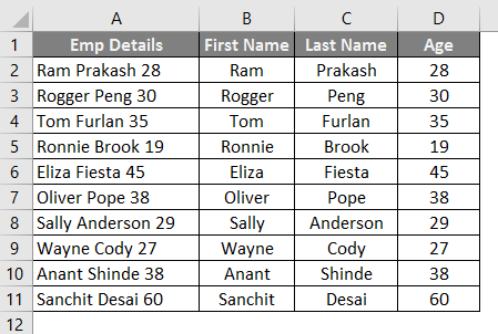
Click on the Finish button. You will see an output as below.
Text to Column can be used as a reverse of the Concatenate function.
Example #2 – Splitting Text using Flash Fill Option in Excel
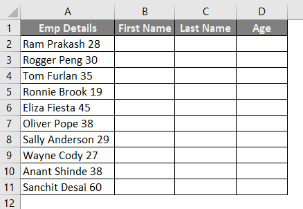
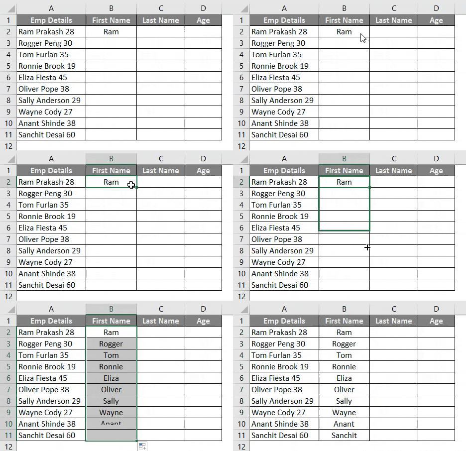
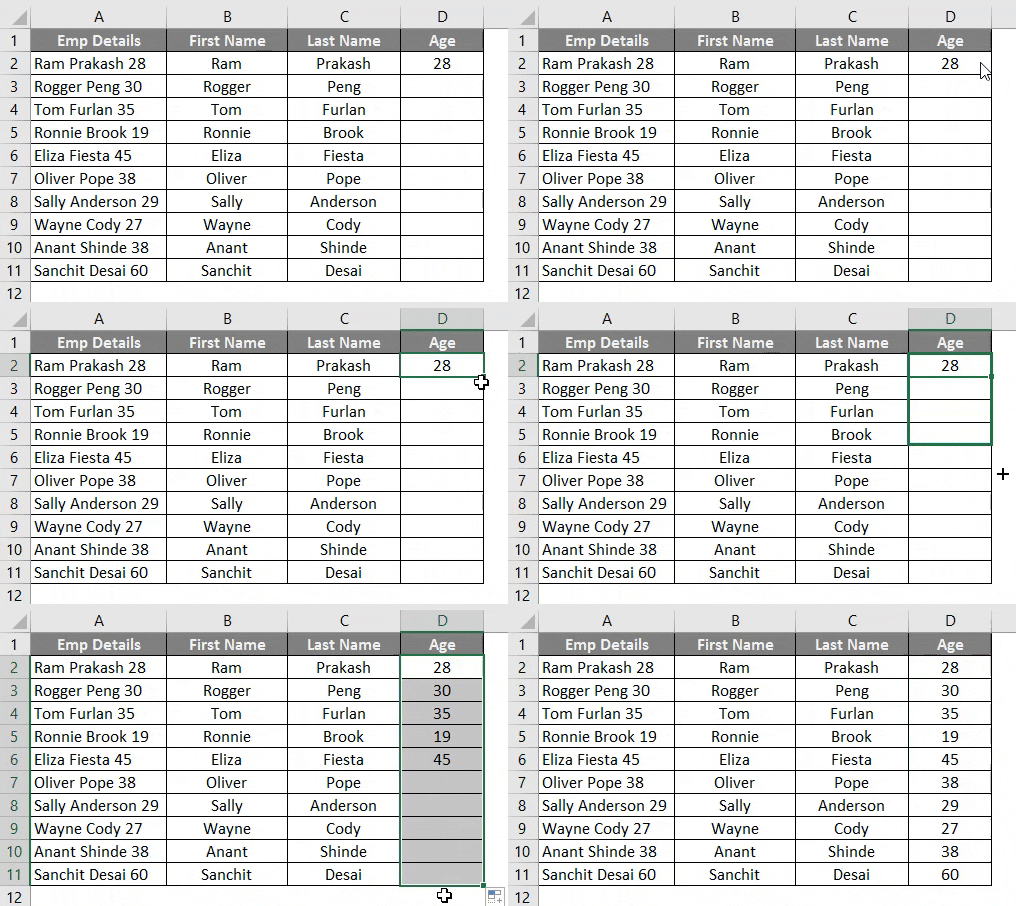
If you use Excel version 2013 or above, one tool is handy for splitting text into different columns. It is called the Flash Fill feature. This tool not only automatically populates the data into other cells but also splits the cell data into different columns. Suppose we have data as shown below. We want First Name, Last Name, and Age in three columns.
- Insert three new columns after the column containing data: First Name, Last Name, and Age.
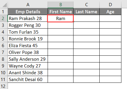
- Under the Column First Name, type the first name as “Ram”.
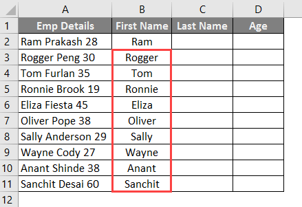
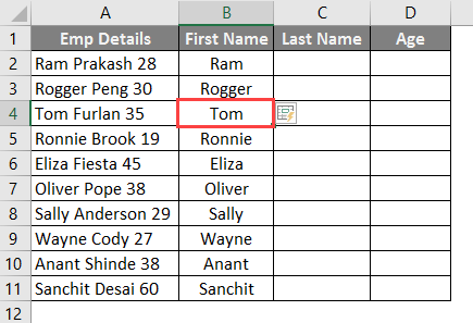
As soon as you type the name “Rogger” in the second cell of column “First Name”, Excel recognizes the pattern and fills all the next cells with the First name. You can see the output below.
- Press the Enter Key.
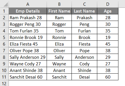
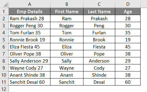
- Do the same procedure for the Last Name and Age columns; your final output will be like the image below.
Example #3 – Splitting Text using Formula
Suppose we have the same data as the previous three examples. We can use the formulae to do the splitting of these text values.
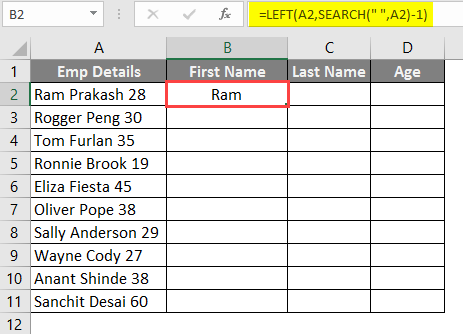
In cell B2, put the LEFT Formula.
Drag the same formula in column B.
In this formula, the LEFT function helps you extract data from the left. The SEARCH function allows you to search the first space (““) from the left-hand side and returns the text in cell B2.
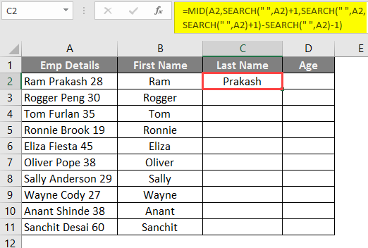
- In cell C2, put the formula as follows and press the Enter Key.
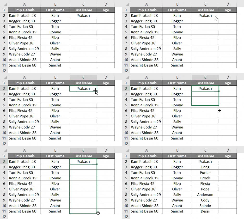
- Drag the same formula in column C.
In this formula, the MID function helps you find the middle value from the text string. The MID function requires three arguments.
- Text within which you want to find the middle value (A2)
- Starting position, which specifies from where the mid function starts extracting the string (SEARCH(“, A2) + 1)
- The number of characters specifies how many characters you wanted to extract from the middle (SEARCH(“, A2, SEARCH(“, A2)+1) – SEARCH(“, A2) – 1).
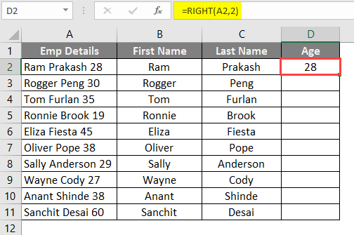
In cell D2, put the RIGHT formula and Press Enter Key.
Drag the same formula in column D.
The Excel RIGHT function allows you to extract the last two characters from the given string in this formula.
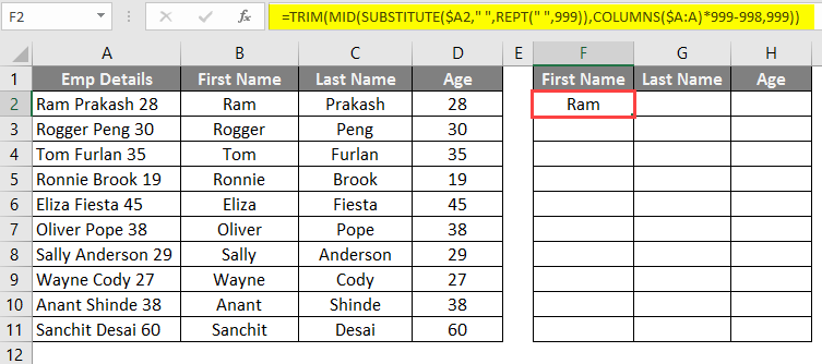
- There is one more formula in which we can do all these calculations in a single shot and save you time. Let’s put the following formula in cell F2 of the current working sheet and see the magic:
=TRIM(MID(SUBSTITUTE($A2,” “,REPT(” “,999)),COLUMNS($A:A)*999-998,999))
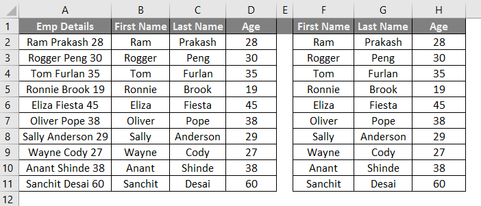
Here in this formula, the only thing that will change is the delimiter value for different cases. Like commas or # in different cases are used, then replace space with these characters. Drag the formula in rows, and you will see the output below:
Things to Remember About the Opposite of Concatenate in Excel
- While working with Text to the column, you must ensure that you select the option of “Treat consecutive delimiters as one“. For example, if you have a name in the format Ram, Prakash, as you can see, there are two delimiters (comma and space); this option will consider comma and space as a single delimiter and will separate the First and Last Name in two different columns. If you do not check this option, it will split the data into three columns with First and Last Names in extreme columns and space as a separate string in one column.
- While working with text to the column, make sure you are selecting the output range properly. By default, the actual cell containing data is selected. If you do not change that, it will replace the original data.
- You can’t give output range from other worksheets while working with text to column method for separating text.
Recommended Articles
This is a guide to Opposite of Concatenate in Excel. Here we discuss How to use the Opposite of Concatenate in Excel, practical examples, and a downloadable Excel template. You can also go through our other suggested articles –
