Updated August 21, 2023

Pivot Table Sort in Excel (Table of Content)
- Pivot Table Sort in Excel
- Steps to Create a Pivot Table in Excel
- How to Sort Pivot Table Columns in Excel?
- How to Sort Pivot Table Rows in Excel?
Pivot Table Sort in Excel
To sort any pivot table, there are 2 ways. First, we can click right on the pivot table field we want to sort and select the appropriate option from the Sort by List. Also, we can choose More Sort Options from the same list to sort more. Another way is by applying the filter in a Pivot table. Go to the cell out of the table and press Shift + Ctrl + L together to apply the filter. Now from the drop-down list, we can choose any Sorting type as required.
Steps to Create a Pivot Table in Excel
A brief discussion below will familiarize you with how to create a Pivot Table in Excel:
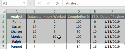
Step 1: Select the table you want to get data from.
Step 2: Click on Insert.
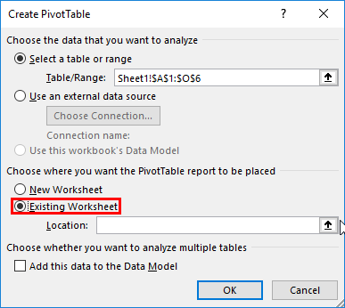
Step 3: Select the Pivot Table, and a pop-up window will appear.
Since we have already selected the data, the Select Table or Range option is auto-filled; it can be done here if you want to change it.
Step 4: Select from where you want the Pivot table to be located; in this case, I am creating a new page but not a new sheet.
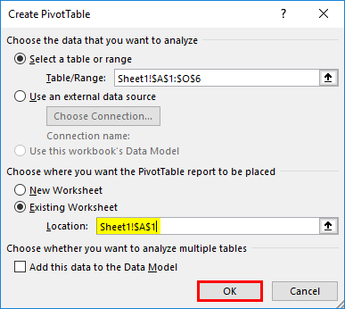
Step 5: Specify the exact location of the Pivot Table.
Click Ok, and your pivot table is now created.
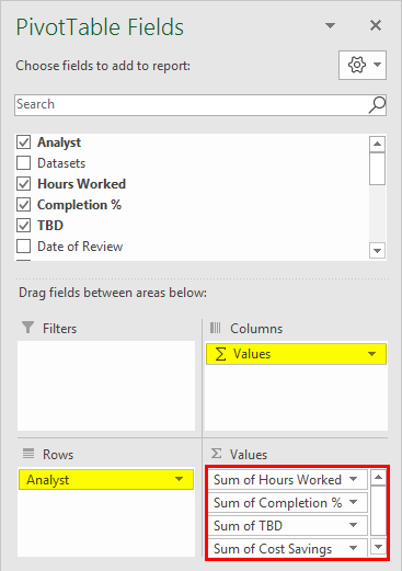
Step 6: Now that the pivot table is created, specify which data you want to display.
The end result should look like this:
I created a small table to illustrate how to create a pivot table. The practice dataset also includes a larger pivot table for you to work on. We have taken these values from it and will use them to illustrate how to sort data in a pivot table.
Now that we have seen how to create a pivot table let us get to this article’s main subject: sorting data inside a pivot table.
How to Sort Pivot Table Columns in Excel?
For small tables, sorting data is straightforward; you just need to select the Row Label column to sort the data alphabetically and specify whether you want to sort from A-Z or Z-A.
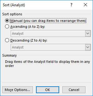
Or you can click More Sort Options to get detailed settings in the pop-up window on the screen.
As you can see, sorting can be done alphabetically from A-Z or Z-A, by value in ascending or descending order, or manually using any order we need for visualizing the data.
For larger tables, perform the following steps:
- Click on Data in the Ribbon Menu at the top of the screen.
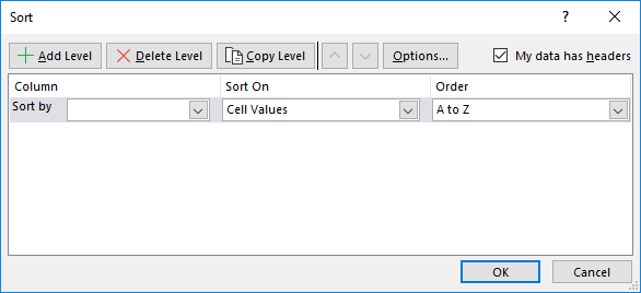
- Click on Sort, and a pop-up window appears.
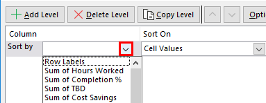
- We can select any of the attributes we want to sort from the table and sort by value, alphabetical order, and many other attributes in the pop-up window.
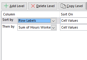
- We can also sort multiple attributes simultaneously by clicking on add level and specifying the next parameter we want to sort.
Returning to our original example, we can now find out who worked, how much, and how much cost savings were available for each employee. We can also find out various parameters for sets of data by sorting according to our preferences and selecting filters accordingly. The result of this would give us the data we require.
How to Sort Pivot Table Rows in Excel?
We have seen how to arrange pivot table data in various orders inside a column. The following steps illustrate how to sort pivot table data inside a row.
Consider the following table:
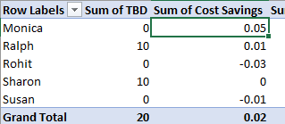
If we want to see the TBD values next to the Analyst Name directly, we need to sort the data in the rows so that the Cost Savings column is next to the Row Labels column.
To do this, perform the following steps:
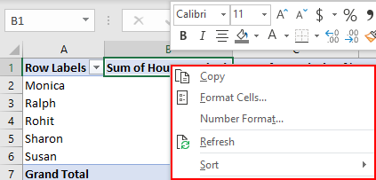
- Right-click on the cell where you need to start sorting from, and a dropdown menu appears:
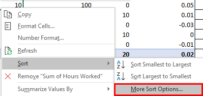
- Select Sort and then More Sort Options from the next dropdown that appears
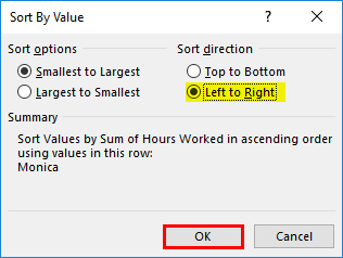
- A pop-up window appears. Select the order which you want, in this case, the smallest to largest order, as we can see from the data:
Select Left to Right instead of Top to Bottom and click OK.
- The end result should look like this:
We have seen examples and learned how to sort data in Pivot.
Things to Remember
- Before sorting any data, ensure no extra spaces are leading the values; these leading spaces will affect sorting results, especially if we sort text values or use text parameters such as sorting alphabetically from A-Z Z-A.
- In pivot tables, sorting cannot be done on a case-sensitive basis for text, all text is treated as the same case, and no distinction is made between uppercase and lowercase.
- Pivot tables do not allow sorting by a specific format, such as cell color, font color, or conditional formatting indicators like sets of icons.
- Sorting in Pivots requires practice and knowledge of the data structure you are working with, as the selection of sorting parameters will depend on this.
- While using multiple sort levels, never select the whole table, as it will change the structure of the pivot and throw an error instead of the desired result.
Conclusion
Data analysis using Excel is a vast field. Pivot table sort is just one of the many features available for us to sort, analyze and display data.
As we keep learning new concepts, we will find new and exciting ways to manipulate data. I have included a practice workbook along with this article. You are encouraged to add your data and apply the concepts highlighted in this article. Further resources are available elsewhere on our website and the Microsoft Support site for specific functionalities.
The key to learning and applying these concepts effectively is practicing with the kind of data an actual business would use, not being afraid to make mistakes, and having an open mind toward different challenges we might face on our learning journey. Teaching new concepts is always a pleasure, and I hope you find our content interesting. Have an enjoyable learning experience.
Recommended Articles
This has been a guide to Pivot Table Sort in Excel. Here we discussed How to Sort Pivot Table Columns and Rows in Excel, Examples, and downloadable Excel templates. You may also look at these useful functions in Excel –
