Introduction to Polyval MATLAB
‘ Polyval ’ is one of the important syntaxes in Matlab because it is very complex to solve mathematical quadratic or linear equations in computer systems. ‘ polyval ’ supports resolving these problems. By using the polyvalent command, we can solve complex polynomials in Matlab. This command is not limited to one or two degrees but evaluates roots of “n” number of degrees and roots. It includes other functions also, such as poly, polymer, poly int, polyvalent, polybag, residue, roots, conv, second, and polyfill; Polyint is a function used to compute the definite integration of polynomials. Polyfit, on the other hand, is used to fit a polynomial of the specified degree to a given set of data points. Polyvalm allows for evaluating matrix-vector polynomials. Polyval is commonly used to evaluate polynomials at specific values.
Syntax:
- Op = polyval(eq1 ,eq2): output variable name = polyval (coefficient of polynomial, points location)
- Op = polyint(eq1): output variable name = polyint(coefficients of polynomial)
- [op,op1] = polyfit(range ,eq1, 1): Output variable names = polyfit (range, polynomial coefficients, 1)
Why we Use Polyval Matlab?
The roots of polynomials can be found using a variety of functions and instructions, but other approaches are unable to assess the roots or solutions of higher-degree polynomials. Polyval is crucial in such situations. If we want to find the roots of polynomials at different locations, we use polyvalent. Let us assume one equation x 1 = 9 x^3 + 5 x^2 + 4 x + 9 at points 4, 5, 3, 2; then, it will create one vector [ 9, 5, 4, 9 ]. This vector represents the coefficients of the polynomial. It also helps to evaluate the definite integral of polynomials. And if we want to fit or use multiple values or ranges, we can use the poly fit command.
Examples to Implement Polyval MATLAB
Below are the examples mentioned:
Example #1
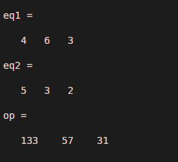
let us consider two equations eq1 = 4 x^2 + 6 x + 3 and eq2 = [ 5, 3, 2 ] , eq2 is location of points . Example 1 shows the Mat lab program to solve this problem. The output of this example will show roots of the above eq1 at locations 5, 3, and 2.
Code:
clc ;

clear all;

eq1 = [ 4, 6, 3 ]
eq2 = [ 5, 3, 2 ]
op = polyval(eq1, eq2)
Output:
Example #2
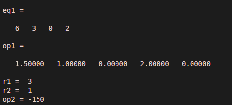
Let us consider the integration example with limits r1 and r2. Eq1 =6 x^3 + 3 x^2 + 2. In eq1, one degree is missing; therefore, we will consider the coefficient as 0. And values of r 1 and r 2 are 3 and 1. To evaluate this problem, first, we will calculate the integration of eq1 by using the polyint command, and after integration, we can find defined values by putting the output and values of r1 and r2 in the polyval command.
Code:
clc ;

clear all ;

eq1 = [ 6, 3, 0, 2 ]
op1 = polyint(eq1)

r1 = 3

r2 = 1

op2 = diff(polyval( op1, [ r1 , r2 ] ))
Output:
Example #3
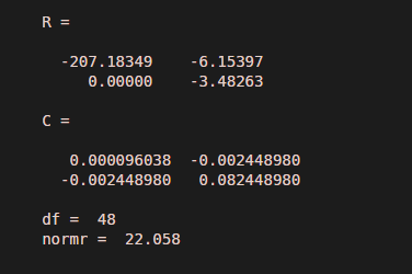
For example 3, we utilized the polyfit function to fit a range of values from 1 to 50 into a first-degree polynomial. The polynomial equation is stored in the variable “equation 1”.After assigning the values, we fit the polynomial and range in function using the polyfit command. Matlab code shows an implementation of example 3
Code:
clc ;

clear all ;

range = 1 : 50 ;

eq1 = 0.5 * range + 3 * randn(1, 50 ) ;

[ op ,op1] = polyfit(range, eq1, 1)
Output:
Conclusion
We have seen polynomial evolution in the above modules using Mat Lab. We can use various commands to find the exact solution, such as polyval, polyint, polyder, poly, and polyfit. We can also evaluate arbitrary polynomial by using these commands. Along with these applications, we can also find higher degree polynomial solutions by using polynomial matrix and polynomial regression .polynomial regression is one of the important applications of polyval implementation.
Recommended Articles
We hope that this EDUCBA information on “Polyval MATLAB” was beneficial to you. You can view EDUCBA’s recommended articles for more information.


