Updated May 8, 2023
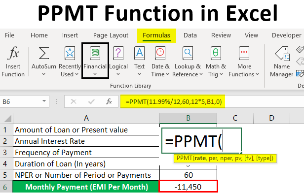
Introduction to PPMT Function in Excel
PPMT is a financial measure to check out the principal amount of a given loan amount. When you pay periodic payments on a loan taken from the bank, a specific amount or part of each payment usually goes towards the interest (it’s a fee charged for borrowing the loan), and the remaining amount of the payment to the principal loan amount (it is the amount you originally have taken or borrowed). In Excel, we can find out both interest & principal amount. PPMT function is used as both worksheet & VBA function. Most commonly used function by bank professionals, financial analysts & consultants in real estate.
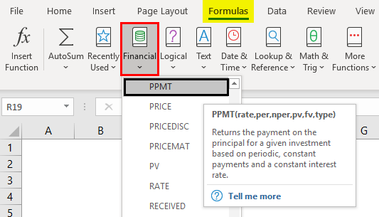
It’s an inbuilt or pre-built integrated function in Excel that is categorized under the Financial function.
Definition of PPMT Function in Excel
PPMT return payment of a principal amount for an investment is based on a periodic, constant payment schedule and a fixed interest rate for a given duration or time. It indicates the principal amount paid in any given pay period.
Syntax of PPMT Function
Arguments for PPMT Function
- Rate: It’s the interest rate of the loan.
- Per (Period): A target or specific payment period; it usually indicates how much the principal amount has been repaid.
- Nper (Number of a payment period): Total number of payments to be made for the loan, i.e., It is the number of payment periods during the timezone of the loan; suppose if payments are monthly for 3 years, this would be entered 3*12 to calculate 36 payment periods.
- PV (Present value): The present value or amount of a loan till now.
- FV (Future value): An optional argument or parameter that indicates the loan’s future value at the end of the last or next payments.
- Type (optional): An optional argument or parameter that indicates when the payments are made, i.e., either at the beginning (1) of a month or at the end (0). If you enter the value 1, payments are due at the beginning of each period. If you enter the value 0 or a blank value, then payments are due at the end of each period.
Note:
- Rate: It should be either entered as a percentage or a decimal number, i.e., if you are making an annual payment at the annual rate of interest of 9%, then it should be entered as 9% OR 0.09 OR monthly payment of the same loan with the same interest rate, then you should enter as 9%/12.
- Per (Period): It should be entered in the 1 to NPER value range.
- FV ( Future Value): If you skip or omit this value, the [fv] value will be 0 by default.
- Type: If you skip or omit this value, the [Type] value will be 0 by default.
How to Use the PPMT Function in Excel?
PPMT Function in Excel is very simple and easy. With some examples, let’s understand how to use the PPMT function in Excel.
Example #1 – Calculate the PPMT Value for a 5 Years Duration of Loan
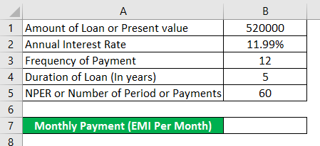
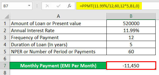
The below-mentioned example contains the below-mentioned details of the loan. Here, I need to determine the principal amount using the PPMT function.
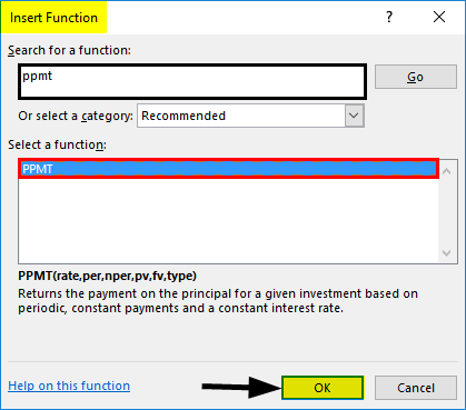
- Now, select the “Insert Function” button (fx) option under the formula toolbar, and a dialog box will appear; in the search for a function text box, you can enter the keyword “PPMT” and click on the go, automatically, function name will appear in “Select a function” box.
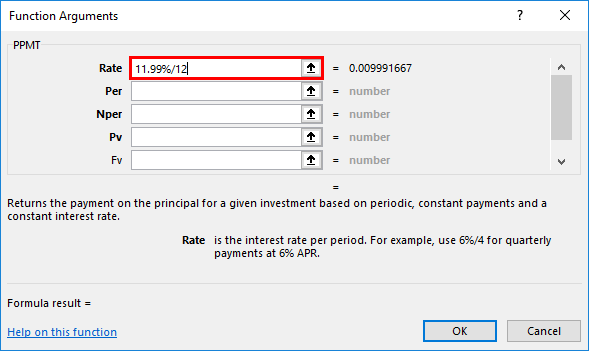
Now, you can double click on the PPMT function in the “Select a function” box. A formula window popup appears where you need to input the formula or syntax argument of the PPMT Function. i.e. =PPMT (rate, per, nper, pv, [fv], [type]).
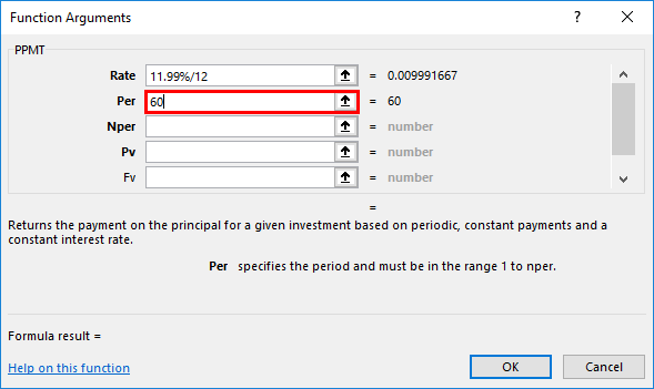
- Rate: It’s an interest rate of a loan; here, the annual interest rate is 11.99%; therefore, we need to enter it as 11.99%/12.
- Per: It’s a target or specific payment period, i.e., here, the period will be 60 months.
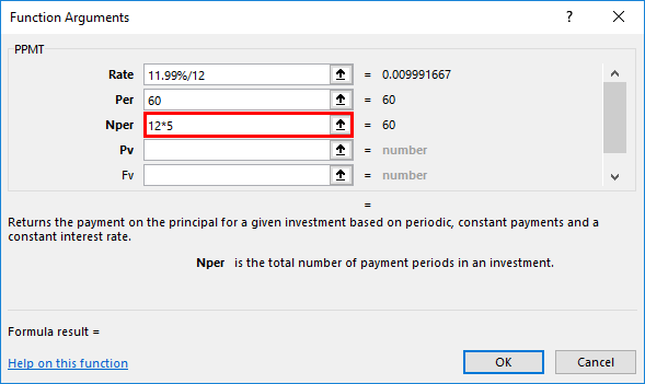
- Nper (Number of a payment period): Total number of payments for the loan; here, the payments are made monthly for 5 years, so it will be 60 months to enter as 12*5.
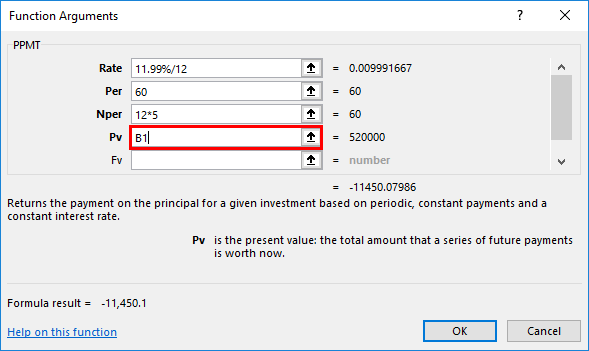
- PV (Present value): It is the present value or amount of the loan; here, you can enter it as a cell reference of the loan amount (C7) or its value of 520000.
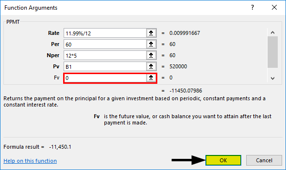
- FV (Future value): It is an optional argument where this parameter can be skipped or omitted; here, you can enter a value as 0 or [fv] value will be 0 by default; we need to assume it as zero balance after the last payment or at the end of NPER payments.
- Once after entering all the arguments, we can click on Ok =PPMT (11.99%/12,60,12*5, C7,0), i.e., returns the PPMT or principle amount or value per month. i.e., -11,450 in cell B7.
Example #2 – Calculate the PPMT Value for a 3 Years Duration of Loan
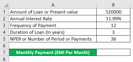
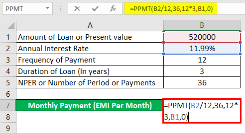
We can calculate the PPMT value for 3 years of the loan; we need to change the PER & NPER values.
Using PPMT Function in Cell B7.
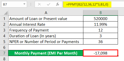
After using the PPMT Function in cell B7, the answer is shown below.
i.e., =PPMT (11.99%/12,36,12*3, B1,0) returns the PPMT value -17,098.
Things to Remember
- If you enter any of the Values or arguments in PPMT as non-numeric, it will result in a “Value error”.
- If the Per (Period) argument in the PPMT function is less than 0 or greater than the NPER value, it returns a “#NUM! error”
- You need to enter the correct cell reference; if it is incorrect, it will return VALUE! error, even if you forget to convert an interest rate or divide the interest rate argument by 12 or 6 0r 4 (based on annual or quarterly payment), it will result in VALUE! error.
Note: It should always be entered in the 1 to NPER.
Recommended Articles
This is a guide to PPMT Function in Excel. Here we discuss How to use the PPMT function in Excel, practical examples, and a downloadable Excel template. You can also go through our other suggested articles –
