Excel Project Management Template (Table of Contents)
Definition of Project Management Template
Project Management Template handles workloads and activities if any changes occur. A project management template is helpful for visualization, planning, organizing, tracking & managing allocated tasks or projects by a client. If anybody asks you, how is the project going on & its progress?
Then you can present the project management template. When you work on any project, you will come across a different phase of the project i.e.
- Initiation phase
- Development phase
- Execution phase
- Monitoring and Controlling Phase
- Deliverance Phase
How to Create a Project Management Template in Excel?
Let’s check out how to create a project management template & how to use it in Excel.
Illustration #1 – Project Task Details & Its Estimated Duration
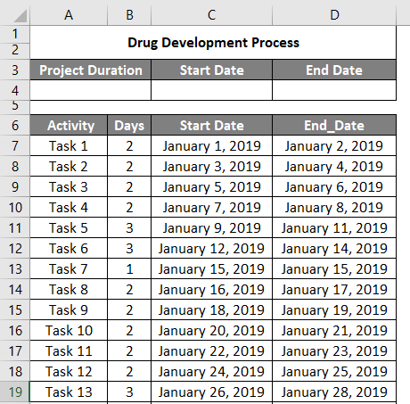
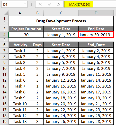
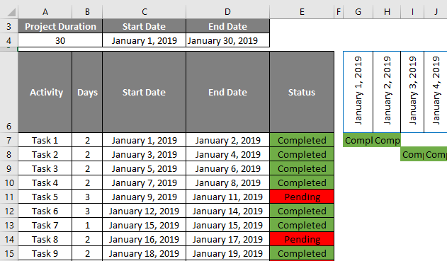
Enter the task details of the project & estimated duration, its start date & end date. The date should be entered in the below-mentioned format for better appearance, and it is applied to both the start date & end date column range.
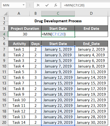
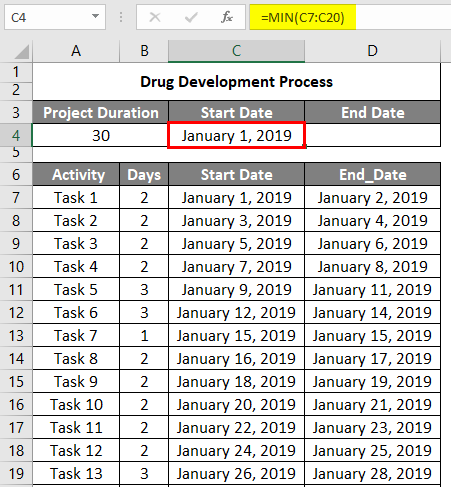
Apply the MIN formula in cell “C4” to get the minimum value under the project start date range.
After using the formula, the output is shown below.
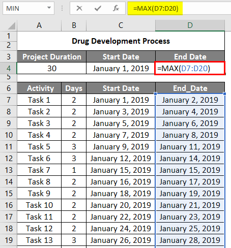
Apply the MAX formula in cell “D4” to get the maximum value under the project End Date range and enter the total project duration.
After using the formula, the output is shown below.
Illustration #2 – Project Timeline Creation
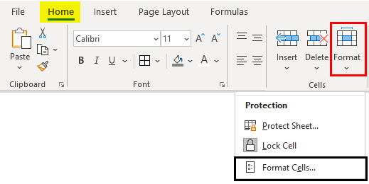
Go to Home >> Format >> Select Format Cells option.
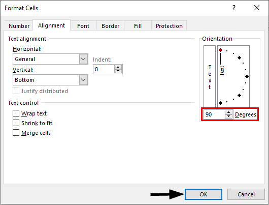
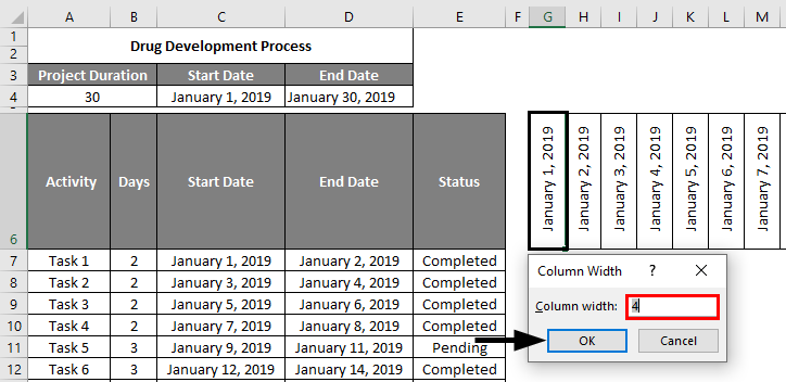
After selecting the Format Cells option, the Format Cells window appears. Now, enter the alignment to a 90-degree orientation & format it in a similar way by dragging that task 1 start date to the last task end date or until you get Jan 30th, 2019.
Set the column width as 4, and the row height is adjusted for a better text content appearance.
Illustration #3 – Formula Explanation (Two Conditions)
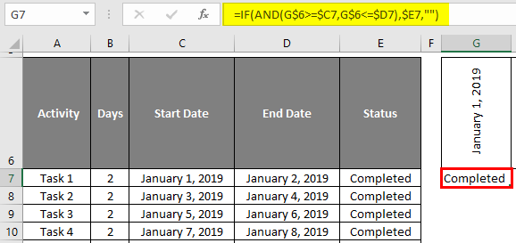
=IF(AND(Jan 1st, 2019>= Jan 1st, 2019, Jan 1st, 2019<=Jan 2nd2019), If yes or if the criteria meet, give the value of status Cell reference or leave it blank).
If I want to apply this formula to a whole date or project range, then I need to modify the formula with mixed reference, i.e., row & column reference modification.
I apply this formula towards other columns on the right-hand side (Other date range). To get an output, I need to lock column C & D (i.e., $C7 & $D7) & the status reference column as well, i.e., column E (“$E7”).
Similarly, I will be dragging this formula down; I need to lock row reference, i.e., 6th row (G$6 & G$6).
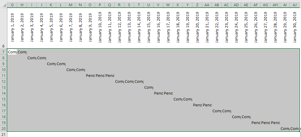
Now, apply this formula to a whole date range, i.e., By selecting the entire date range, you need to press CTRL+R & CTRL+D keys. So that it gives status reference values if the IF logical condition criteria meet.
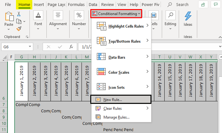
Make the text alignment of the date range to the center and remove the gridlines & table borders. Now, select the entire date range & apply conditional formatting to the date range by applying a new rule.
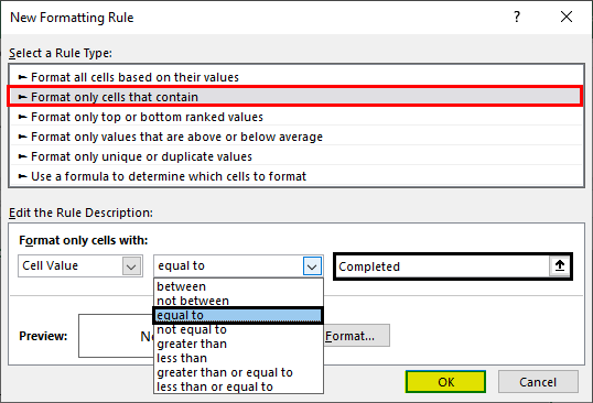
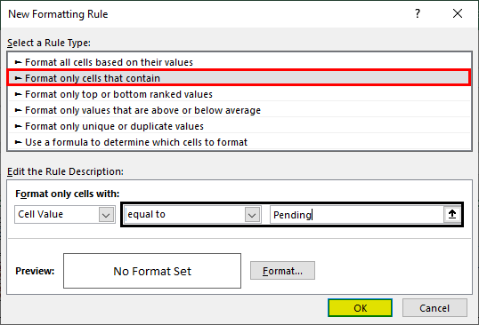
Under the New Formatting Rule, select “Format only cells that contain” under the cell values, select equal to enter the keyword “Completed”, and click on the format option for color selection.
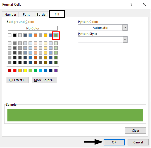
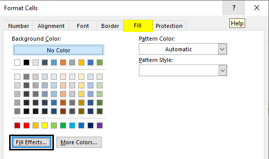
In the format cell, click on Fill; under that, select Green color, and click OK. Now the cells which contain completed will appear in green color.
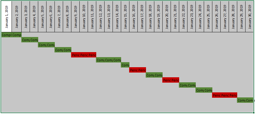
After selecting a color, the output is shown below.
Similarly, under New Formatting Rule, select “Format only cells that contain”, under the cell values, select “equal to,” and enter the keyword “Pending”, click on the format option for color selection.
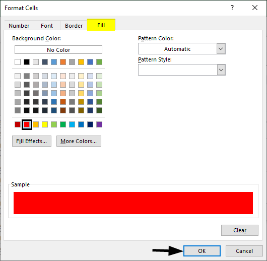
In the Format Cell, click on Fill; under that, select red color, and click OK.
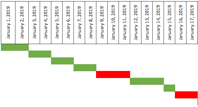
Now, the cells which contain completed will appear in red.
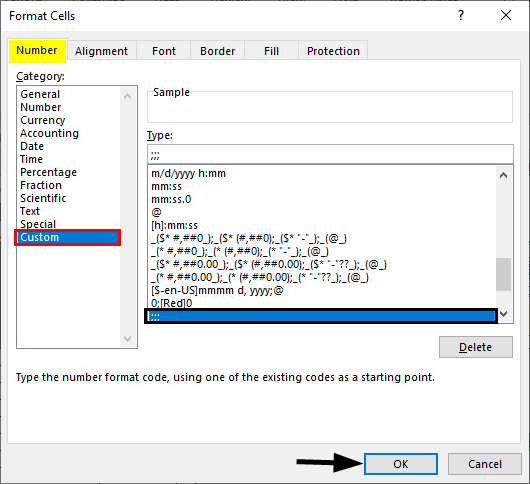
Now, I need to remove the text content on the color bars. It can do this by selecting the entire date range of color bars and right-clicking the Format Cells option. Under that, select “Custom” in the category of number format, enter a semicolon three times under “Type,” and click OK.
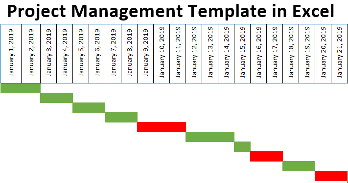
Now, you can observe only colored data bars appear.
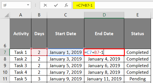
Now, the date range color bars need to be linked with the end date of each task; this needs to be done because once you complete the pending task in the activity list, the task’s duration needs to be entered. If you join or update the end date & duration of a task, the color bar width automatically changes based on the completion date you enter.
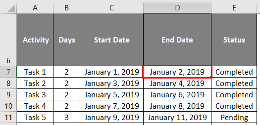
After applying the formula, the output is shown below.
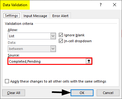
Simultaneously you can create & apply a data validation list to the status range; by selecting the complete status range, press ALT+D+L so that the “Data Validation” popup appears under the “Validation criteria” in the “Allow” dropdown, select “List” and in the source enter the two status parameters, i.e., “Completed & Pending” separated by a comma.
Now, clicking on any status parameters lets you observe the dropdown list. If you change from pending to completed, color changes are observed in color bars.
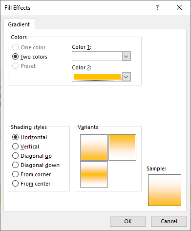
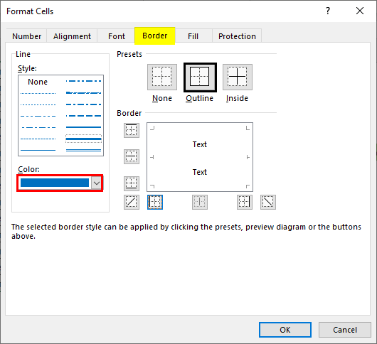
You can format the task table for a better appearance with the dual color tone and apply a border to the project plan.
You can apply conditional formatting to the status parameter range, with green color for the cell containing the keyword “Completed” & red color for the cell containing “Pending” so that you will come to know the status of each task.
Things to Remember about Project Management Template in Excel
- It outlines the goals and objectives of each task with an actual planned start date, actual executed start date & estimated end date, or the due date of It.
- It also helps quantify the resource requirements for the allocated task and determine budgets and timelines for each task & its completion.
- Gantt Chart also uses for preparing and track a project plan.
- IF logical test & Conditional Formatting is most commonly used to prepare a comprehensive project plan.
Recommended Articles
This is a guide to Project Management Templates in Excel. Here we discuss how to create a project management template in Excel, practical examples, and a downloadable Excel template. You can also go through our other suggested articles to learn more –
