Updated May 30, 2023
PROPER Function in Excel (Table of Contents)
PROPER in Excel
A proper function in Excel is used when we have a string of text or a sentence not in a proper format. This function considers only text as an input. Using the Proper function here will convert that text into a proper case in which every word’s first letter will be in CAPS or Upper case, and the rest of the letter will be in Lower case. For example, we have a text as “this is a bat“, then using a proper function, it will change its format as “This Is A Bat.”
It is a built-in function of Microsoft Excel.
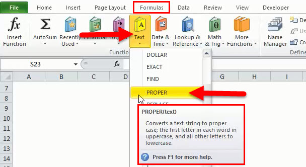
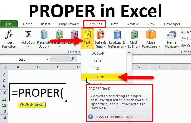
We can refer above picture to know where a PROPER in Excel is exactly located. Firstly, we have to go to Formulas, and under this head, we have to click on PROPER.
The PROPER function also helps, or it can also use to set each word in a given string in UPPERCASE. So, we can say that the PROPER function helps to set the text in a proper format. If space is not properly given or there is an unnecessary blank, in that case, also PROPER function helps.
PROPER Formula in Excel:
Below is the PROPER Formula in Excel:
Compulsory Parameter:
Text: In the PROPER function, there is only one parameter: text; we can define it as the cell address for which the PROPER function will be used and converted into the first character in uppercase and the rest in lowercase for each word.
It is very much easy to use and used where the text is messed up for many reasons.
How to Use the PROPER Function in Excel?
PROPER in Excel is very simple to use. Let us now see how to use a PROPER function in Excel with the help of some examples.
Example #1
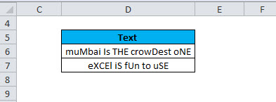
We can take an example of the above one where the Text is not in a proper format; the uppercase and lowercase are mixed, which is wrong. So, doing it manually for big data will take lots of time because it is very difficult to go into each word to correct it. Here, the PROPER function helps to arrange the case in the proper format.
We have two options to do it, i.e., 1) we can do it manually by clicking the PROPER function 2) we can also put a formula in the required cell. We will see it one by one.
Step 1: Click on the cell where we require the proper text.
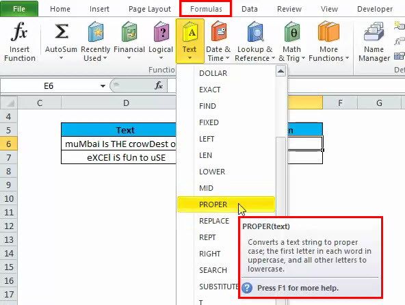
So, in the above example, we want the proper data in the cell address E6, hence clicking on this cell. We can see that it is highlighted in red.
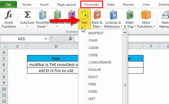
Step 2: Now, we have to go on Formulas in the top ribbon and then click on Text. Below is the picture for reference:
Step 3: After clicking on Text, we have many options or functions to use; then, we will look for PROPER, which is required here and click on that PROPER function. Below is the picture:
After moving to PROPER, we can see that the description of the PROPER function is also given in the box, which says that it “converts a text string to a proper case; the first letter in each word to uppercase, and all other letters to lowercase”.
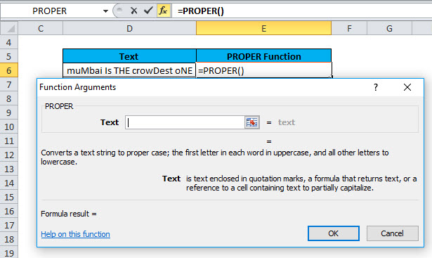
Step 4: Now, we have to click on PROPER, then we will have the below screen:
So, we can see in the above pic that a box appears after clicking PROPER.
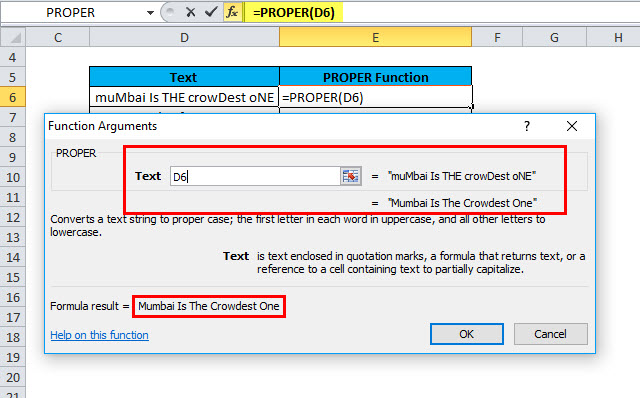
Step 5: We have to put the cell address in the above blank box. It means, as per the formula, we have to enter the Text parameter, so it is the cell address for which we want to apply the PROPER function.
As per this example, the cell address is D6.
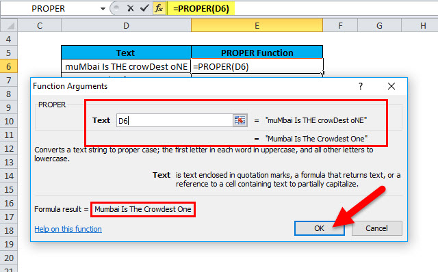
Step 6: We have to finally hit the Enter button or click OK to apply the PROPER function in the given cell address. Below is the picture for reference:
After clicking OK, we will have the result for the PROPER function:
We can see in the above picture that the PROPER function is applied on the D6, and we have the result in the cell address E6. So, in E6, the text is written in a proper format. We can see the first letter of each word is in uppercase, and the rest is in lowercase.
We can drag the formula or copy-paste the formula into the required cell.
Example #2
We have seen in the above example how to apply the PROPER formula manually; now, we will see how to use the PROPER function by just entering the formula in the required cell.
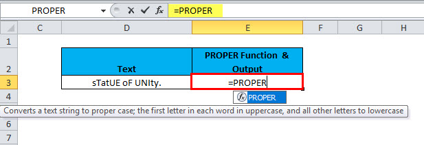
Step 1: In the above picture, we want to apply the formula in E3 for the text available in D3.
So, just type =PROPER.
Step 2: Now, press the TAB button on the keyboard.
Below is the picture for reference:
Step 3: Now, we can see that it is asking for the compulsory parameter, which is text, so we can enter the cell address for which we have to apply the PROPER function. In this case, the cell address is D3. So, we will select the cell address manually or by typing the cell address. Below is the picture:
Step 4: Now, we must close the formula by entering”) “or hitting Enter on the keyboard.
We have the below result:
Things to Remember
- The proper function always converts the’s to S, so it considers the first letter.
The result will be:
We can see in the above pic that after using the PROPER function, it is Excel’S Formula, and the raw data in the cell address is Excel formula. So, we have the proper text with the character in Uppercase and the rest in lowercase. So, always take care of that and convert it manually if “‘” is available.
- The PROPER function affects the numbers and punctuations in the string in which the formula is applied.
Recommended Articles
This has been a guide to PROPER in Excel. Here we discuss the PROPER Formula, how to use the PROPER function in Excel, and practical examples and a downloadable Excel template. You can also go through our other suggested articles –
