Updated February 28, 2023

Introduction to Quiver Matlab
Plots are the means of explaining the insights of any particular topic to the uninformed audience. There are various types of plots that are used in Matlab for various business requirements. Quiver Plot is a two dimensional plot which display the vector lines in the form of various arrows. They are helpful in electrical and mechanical field to show the electric potential and various stress gradients. They can be plotted with the help of one arrow, two arrows, using a mesh grid and gradient.
Functions of Quiver in Matlab
In Matlab, we can plot quiver or velocity plot with the help of function quiver (). Please find the below syntaxes that are used in Matlab to display quiver or velocity plot:
- Q=quiver (x, y, a, b): This syntax is used to plot different vectors in the form of arrows in the different coordinates mentioned in the form if pair in x and y. x, y, a and b matrices must be in the same size and they should contain both velocity and position components. In the resultant plot, arrows are always pointed towards top, however they can be scaled longer or shorter depending on the requirements.
- Q=quiver (a, b): This syntax will draw the vectors that are given in a and b where the points are spaced equally in x-y plane.
- Q=quiver (……, scale): This syntax is used to scale the output or resultant plot which means it will scale the arrows in the plot to fit within the respective grid and if required we can also adjust the arrows by a factor known as “scale”. If scale is given as 2 then the arrows will be doubled of their original length and if scale is given as 0.5 then the arrows will be halved the original length. If we want the arrows not to be scaled, then we can mention scale as 0. We can also adjust the length of the arrows with the help of Length Slider.
- Q=quiver (…., Line specification): This syntax is used to change the properties of the line by line specification like line style, marker symbol, etc. If we want to change the symbol of the marker, then it starts from the origin of the vector.
- Q=quiver (……, Name of the property, Value of the property……): We can use this syntax if we want to modify the properties of the plot. The property name can be mentioned with the required value.
- Q=quiver (axes mentioned,.): This syntax is used if we want to display the plot in the axes mentioned rather than the current axes.
Properties of Quiver Matlab
There are various properties of Quiver Plot in Matlab which are discussed below:
- Arrow color can be modified by ‘Color’ property with the respective values. The values can be in the form of hexadecimal color code, RGB triplet value or a color name.RGB triplet value is an element vector which consists of three elements and it decides the intensity levels of red, green and blue. There can be different colors like red, green, blue, yellow, cyan, magenta, yellow, white and none. There is another property which is associated with Color i.e. ColorMode. It has two values which are auto and manual. If the value is set to auto, then Matlab will control the property of color and if the value is set to manual then we can select the color manually. Auto is the default value of the Colormode property.
- LineStyle is another property which is used to modify the stem of the arrow attached to it. There can be various line styles like solid line(default), dotted line, dashed line, dash-dotted line. LineStyleMode is another property which is used to control how LineStyle is set. It has two values i.e. auto and manual. If the value is auto, then Matlab will set the line style and of it is manual then we can change the style of the line. Linewidth is another property of Quiver Plot which is used to change the width of the stem attached to the arrow. The value of line width should be a positive value and 0.5 is the default width.
- ShowArrorHead is one of the property of Quiver plot which give us the preference to choose whether to show or hide the arrow head. It has two values that are on and off. If the value is set to on(default), then it will show the vector with arrows and if it is set to off then it will show the vectors without any arrow head. MaxHeadSize decides the maximum size of the head of the arrow attached to the vector. It is specified as a scalar value with 0.2 being the default value for it. The data types that are accepted are single, double, uint8, int8, uint16, int16, uint32, int32, uint64, int64.
Examples of Quiver Matlab
Please find the below examples that show the use of quiver in Matlab:
Example #1
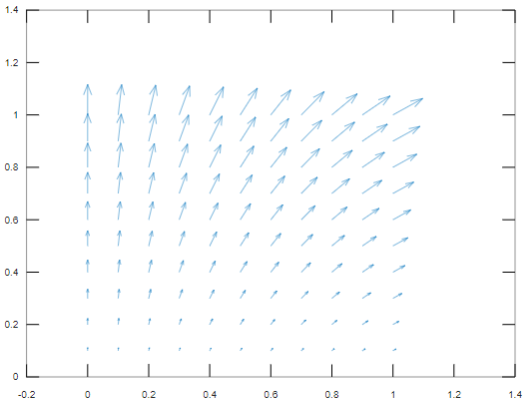
To display the arrows for each data point.
Code:
[x,y] = meshgrid(0:0.1:1,0:0.1:1);

a = sin(x).*y;

b = cos(x).*y;

figure

quiver(x,y,a,b)
Output:
Example #2
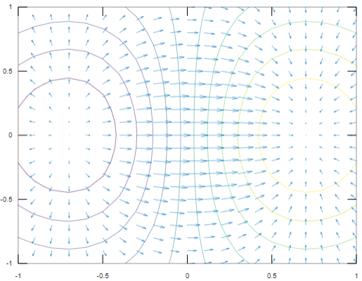
To display the gradient with the Quiver Plot.
Code:
[A,B] = meshgrid(-1:.1:1);

Z = A.*exp(-A.^2 - B.^2);

[GA,GB] = gradient(Z,.1,.1);

figure

contour(A,B,Z)

hold on

quiver(A,B,GA,GB)

hold off
Output:
Example #3
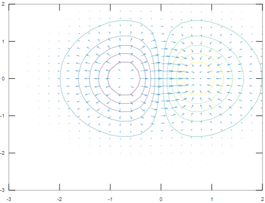
To display the gradient with the Quiver Plot.
Code:
[A,B] = meshgrid(-3:.2:2);

Z = A.*exp(-A.^2 - B.^2);

[GA,GB] = gradient(Z,.3,.3);

figure

contour(A,B,Z)

hold on

quiver(A,B,GA,GB)

hold off
Output:
AutoScale is another property of Quiver Plot which will automatically scale the length of the arrows. It has two values which are on and off. If the value is on, then it will automatically scale the length such that it remains within the grid and if the value is off then it will not scale the length of arrows.
Conclusion
There are various other properties that are associated with Quiver or velocity plot in Matlab. All the properties should be understood to customize the appearance of Quiver plots. They are mostly used in the field of Physics and Mechanics.
Recommended Articles
This is a guide to Quiver Matlab. Here we discuss the Introduction to Quiver Matlab and the various properties along with working and its examples. You can also go through our suggested articles to learn more –


