Updated August 10, 2023
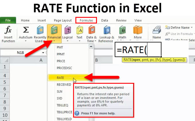
RATE Function (Table of Contents)
Introduction to the RATE Function in Excel
Let’s assume an example. Ram wants to take a loan/borrow some money or invest some money from a financial company XYZ. The company needs to do some financial calculations, like the customer having to pay something to the financial company against the loan amount or how much the customer needs to invest so that after some time, they can get this small amount of money.
In these scenarios, Excel has the most important function, “RATE”, which is part of a financial function.
What is the RATE Function?
A function that is used to calculate the interest rate for paying the specified amount of a loan or to get the specified amount of an investment after some period of time is called the RATE function.
RATE Formula in Excel
Below is the RATE Formula:
The RATE function uses the below arguments
Nper: The total no. of periods for the loan or an investment.
Pmt: The payment made each period, and this is a fixed amount during the loan or investment.
Pv: The current (Present) value of a loan/an investment.
[Fv]: That’s the optional argument. This specifies the future value of the loan /investment at the end of the total no. of payments (nper) payments.
If don’t provide any value, then it automatically considers fv=0.
[type]: This is also an optional argument. It takes logical values 0 or 1.
1 = If payment is made at the beginning of the period.
0 = If payment is made at the end of the period.
If don’t provide any value, then it automatically considers it as 0.
[guess]: An initial guess for what the rate will be. If don’t provide any value, then it automatically considers this as 0.1 (10% ).
Explanation of RATE Function
The RATE Function is used in different-different scenarios:
- PMT (Payment)
- PV (Present Value)
- FV (Future Value)
- NPER (No. of periods)
- IPMT (Interest payment)
How to use the RATE Function in Excel?
The RATE Function is very simple to use. Let us now see how to use the RATE function in Excel with the help of some examples.
Example #1
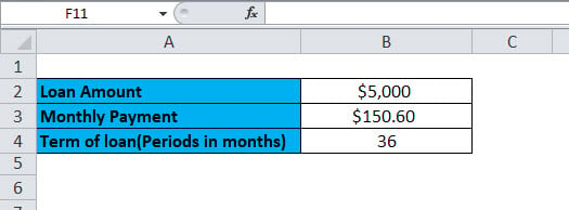
You want to buy a car. For this, you apply for a loan of $5,000 from the bank. The bank provides this loan for 5 years and fixed the monthly payment amount of $150.60. Now you need to know the annual interest rate.
Here, we have the following information available:
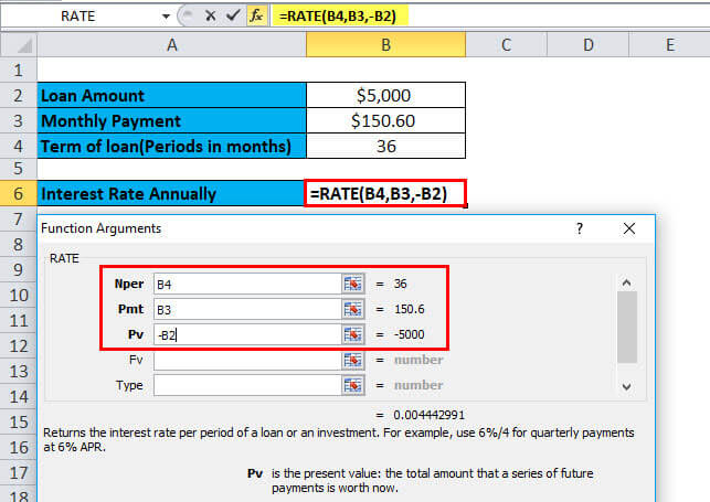
=RATE (B4, B3,-B2)
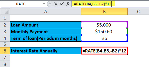
Here the result of the function is multiplied by 12, which gives the annual percentage rate. B2 is a negative value because this is an outgoing payment.
=RATE (B4,B3,-B2)*12
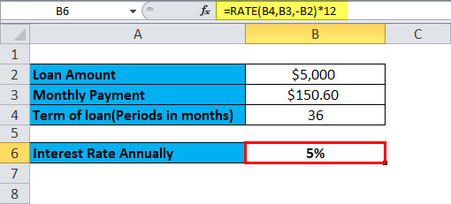
The annual percentage rate will be:
PMT (Payment)
This function is used to calculate the payment made every month for a loan or an investment on the basis of a fixed payment and a constant rate of interest.
PMT Formula:
Example #2
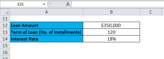
You want to buy a house that costs $350,000. To buy this, you want to apply for a bank loan. The bank offers you the loan at an 18% annual interest rate for 10 years. Now you need to calculate the monthly installment or payment of this loan.
Here, we have the following information available:
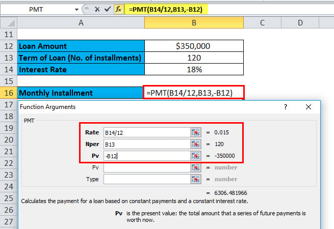
The interest rate is given annually, hence divided by 12 to convert to a monthly interest rate.
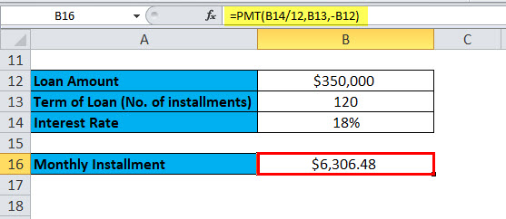
=PMT (B14/12,B13,-B12)
The result will be:
PV (Present Value)
This function calculates the present value of an investment or a loan taken at a fixed interest rate. Or in other words, it calculates the current value with constant payments, a future value, or the investment goal.
Example #3
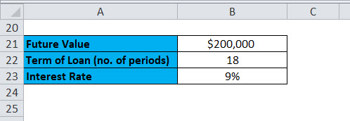
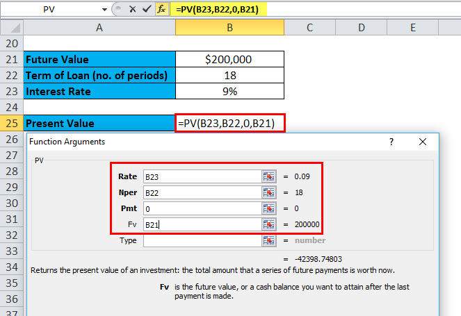
You have made an investment that pays you $200,000 after 18 years at an annual interest of 9%. Now you need to find out how much to be invested today to get a future value of $200,000.
Here, we have the following information available:
=PV (B23,B22,0,B21)
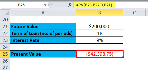
Result is:
The result is in negative numbers as it’s the cash inflow or incoming payments.
Let’s take one more example of the PV function.
Example #4
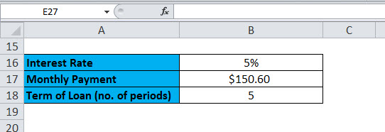
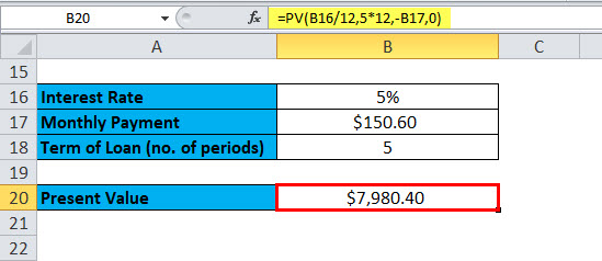
You have taken a loan for 5 years that has a fixed monthly payment of $150.60. The annual interest rate is 5%. Now you need to calculate the original loan amount.
Here, we have the following information available:
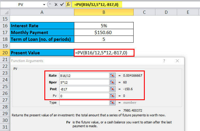
=PV (5/12,5*12,-B17,0)
Result is:
This monthly payment was rounded to the nearest penny.
FV (Future Value)
This function is used to determine the future value of an investment.
Example #5
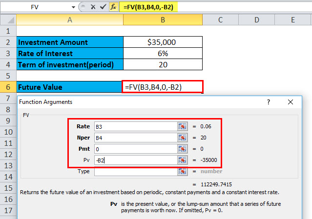
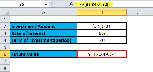
You invest a certain amount of money, $35,000, at 6% annual interest for 20 years. Now, how much will we get after 20 years with this investment?
Here, we have the following information available:
=FV (B3,B4,0,-B2)
Result is :
NPER (No. of periods)
This function returns the total no. of periods for invhttps://www.educba.com/nper-function-in-excel/stment or for a loan.
NPER Formula:
Example #6
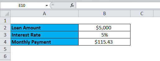
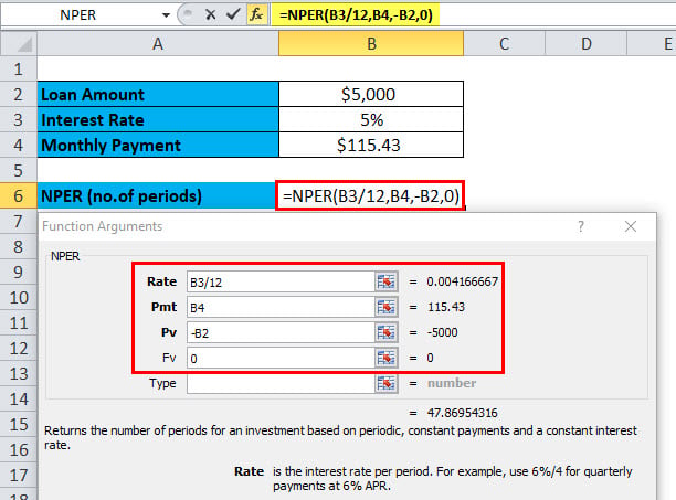
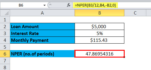
You take a loan of $5,000 with a monthly payment of $ 115.43. The loan has a 5% annual interest rate. We need to use the NPER function to calculate the no. of periods.
Here, we have the following information available:
=NPER (B3/12,B4,-B2,0)
This function returns 47.869 i.e. 48 months.
IPMT (Interest payment)
This function returns the interest payment of a loan payment or an investment for a specific time period.
IPMT Formula
Example #7
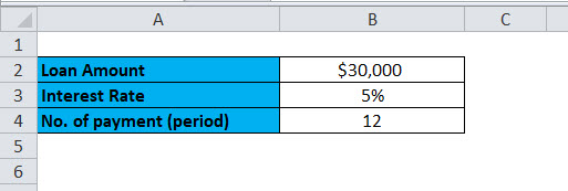
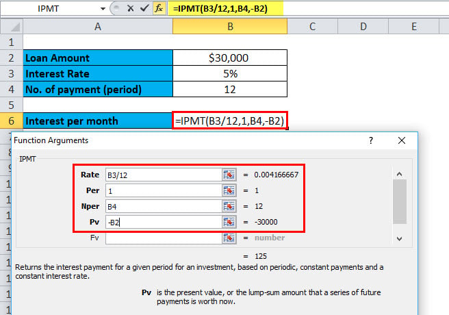
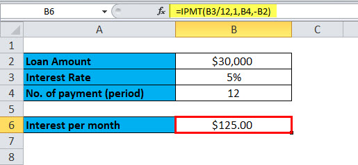
You have taken a loan of $30,000 for one year at an annual interest rate of 5%. Now to calculate the interest rate for the first month, we will use the IPMT function.
Here, we have the following information available:
=IPMT(B3/12,1,B4,-B2)
Result is:
Things to Remember
Two factors are commonly used by the finance industry – Cash outflow & Cash inflow.
Cash outflow: Negative numbers denote the outgoing payments.
Cash inflow: Positive numbers denote the incoming payments.
Recommended Articles
This has been a guide to the Excel RATE function. Here we discuss the RATE Formula and how to use the RATE function along with practical examples and a downloadable Excel template. You can also go through our other suggested articles –

