Updated July 3, 2023
What is the Remove Duplicates in Excel Feature?
Remove Duplicates is an Excel feature that searches for repeated data in the selected cell range and performs the delete operation to provide a data set with unique values.
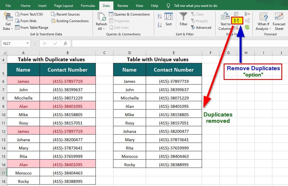
For example, the image below illustrates a table with multiple entries for James and Alan. When we use the Remove Duplicates feature in Excel, we get the table with unique values.
This feature can remove duplicates from a large accounting database while preparing sales reports or data with repeated entries.
Key Highlights
- We can use conditional formatting to highlight duplicate values.
- To remove duplicates, we must filter the highlighted values and manually delete them.
- The Remove Duplicates in Excel feature permanently deletes (removes) duplicate values from a worksheet.
- Excel cannot find and remove duplicates from the area section of a Pivot Table report
How to Remove Duplicates in Excel?
#1 Using Conditional Formatting
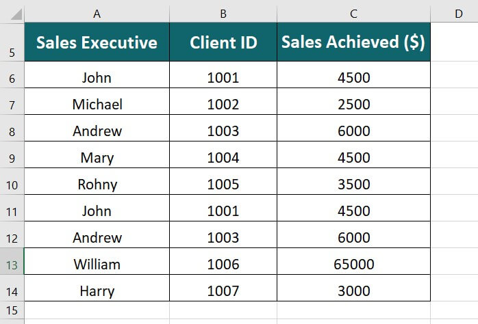
The table below shows the names of Sales executives, their Client IDs, and sales. We want to find any duplicate values in the data using conditional formatting.
Solution:
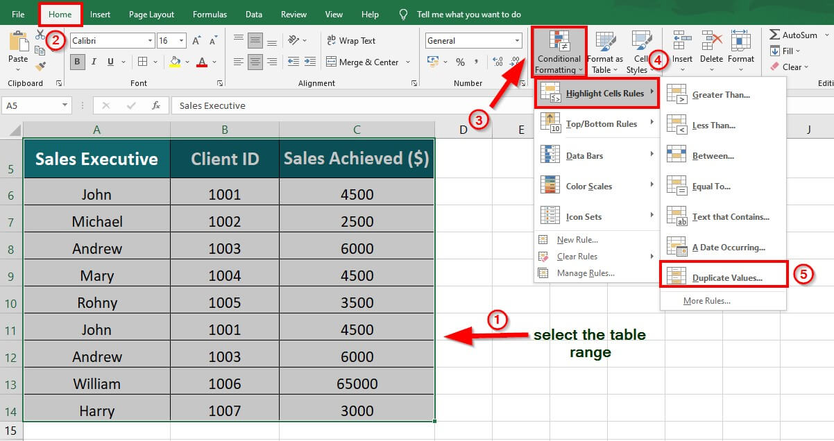
Step 1: Select the data table
Step 2: Go to the Home Tab
Step 3: Go to Conditional formatting > Highlight Cells Rules > Duplicate Values
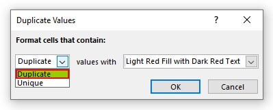
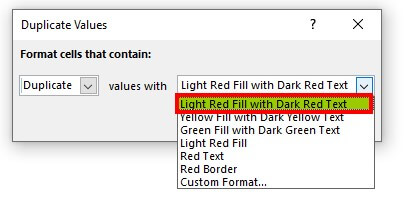
A Duplicate values dialog box will appear
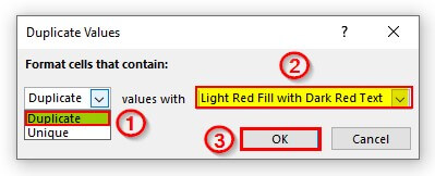
Step 4: Select Duplicate from the drop-down list as shown below
Step 5: Choose the desired highlight color
Step 6: Click on OK
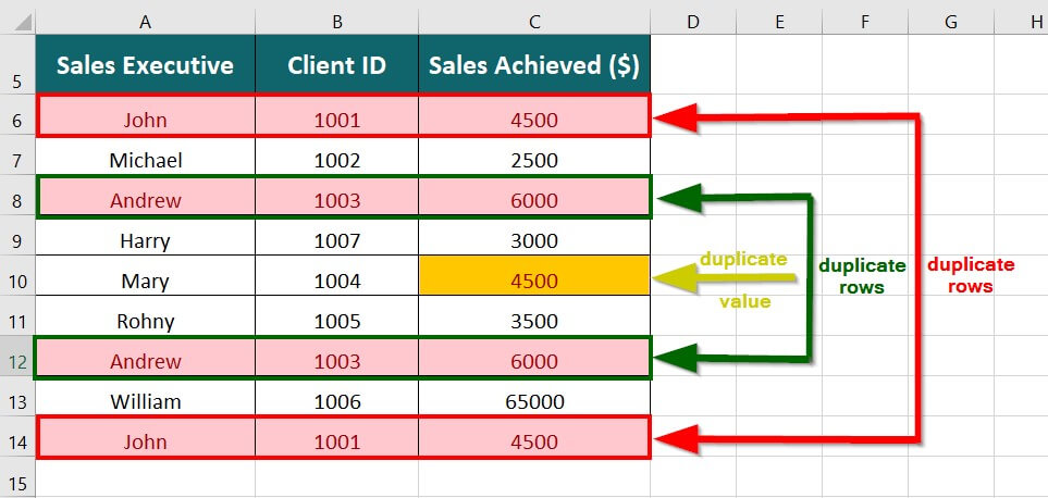
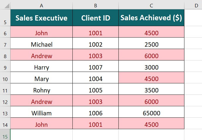
The duplicate values are highlighted as shown below
#2 Using the Filter Option to Remove Duplicates in Excel
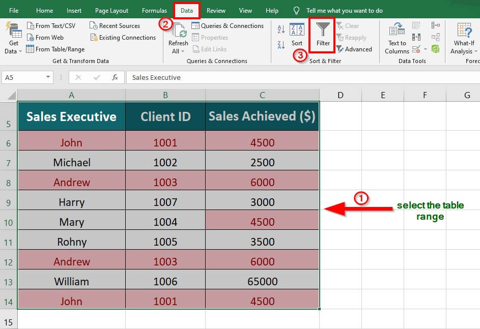
The below table shows highlighted duplicate values. To remove the duplicate rows, follow the given steps.
Step 1: Select the data table
Step 2: Go to Data Tab
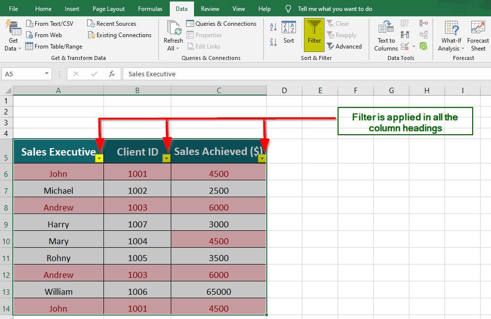
Step 3: Under the Sort & Filter Group, select the Filter option
A filter is applied to all the columns
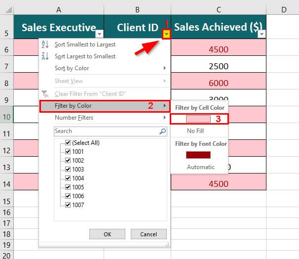
Step 4: Click the filter icon of column B (Client ID)
Step 5: Click on Filter by Color
Step 6: Select Filter by Cell Color
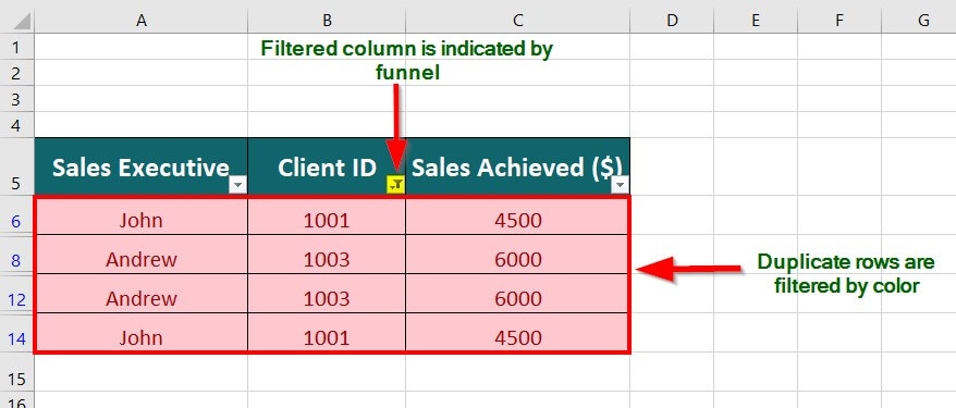
The highlighted (duplicate) rows are filtered as shown below
Step 7: Delete the duplicate rows manually to get Unique values
#3 Using the Remove Duplicates Feature in Excel
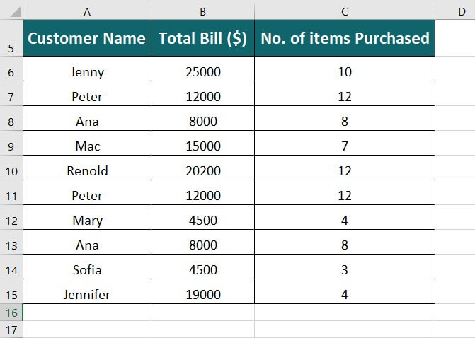
The table below displays a list of customers, their Total Bill, and the number of items purchased. We want to remove duplicate entries from the list using the Remove Duplicates feature.
Solution:
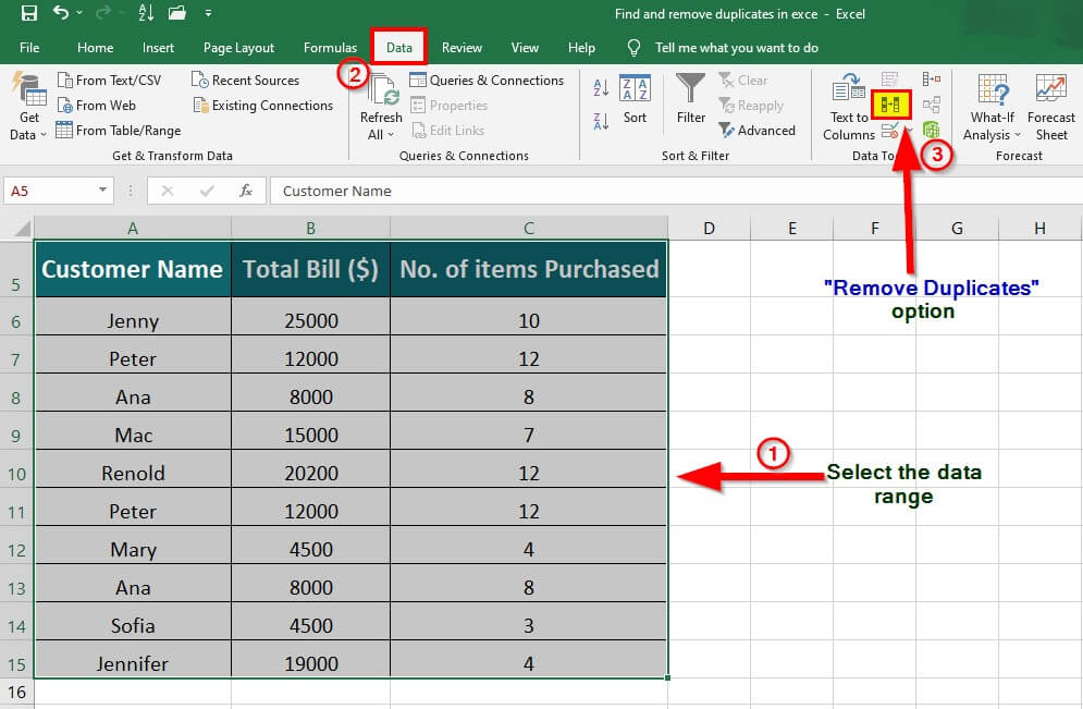
Step 1: Select the data table
Step 2: Go to Data Tab
Step 3: Click the Remove Duplicates icon under the Data Tools Tab.
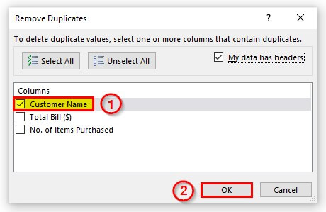
A Remove Duplicates dialog box appears.
Step 4: Select the column headings (customer Name) by which the duplicate value needs to be searched
Step 5: Click OK
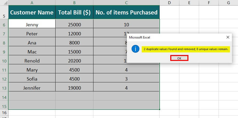
A Microsoft Excel pop-up indicates the number of duplicate values found and removed; and the number of remaining unique values.
Step 6: Click OK
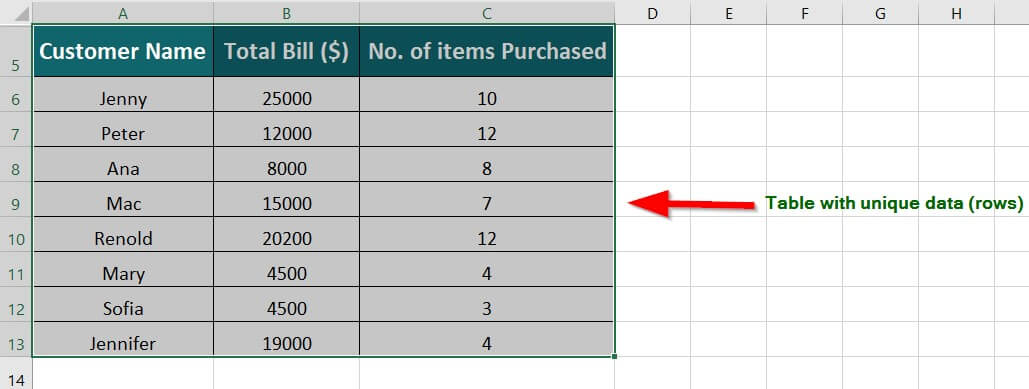
All the duplicate values are removed, and the table now consists of unique values.
#4 Using the COUNTIF Function to Find the Number of Duplicates
We can find the number of duplicate values in a given data set using the COUNTIF in Excel. Consider the following example to understand how it works.
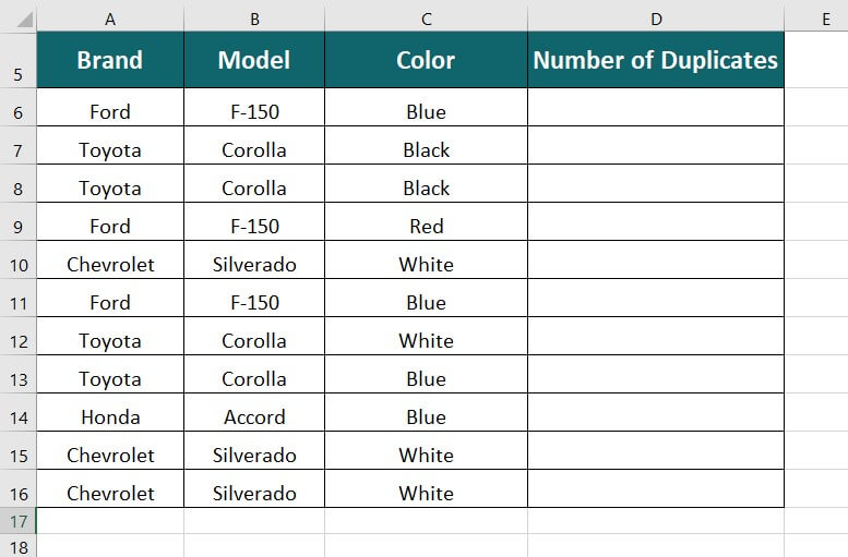
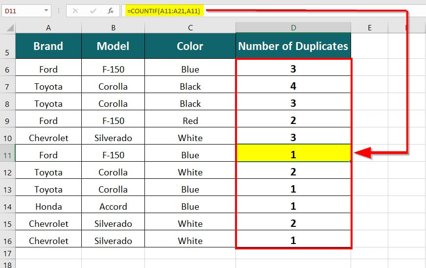
The table below shows the Brand names of four-wheelers with the Model name and colors. We want to find the number of duplicate values using the COUNTIF function in Excel.
Solution:
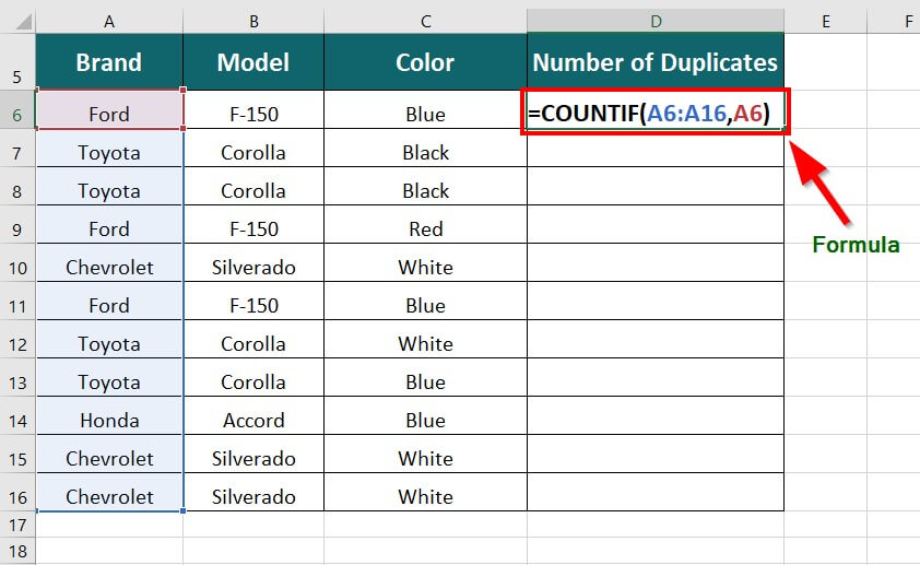
Step1: Place the cursor in cell D6 and enter the formula,
=COUNTIF(A6:A16, A6)
- A6:A16 – It is the range across which we want to find the duplicate data
- A6 – It indicates the first value in the range A6:A16
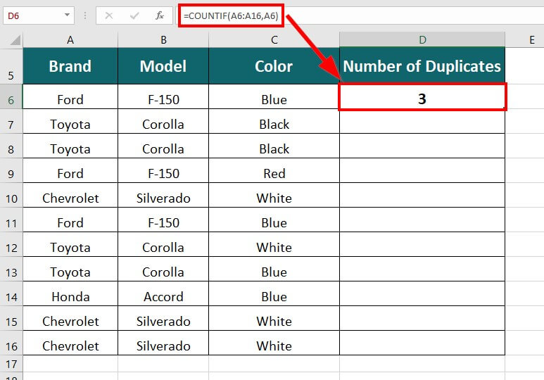
Step 2: Press Enter key to get the total number of duplicates (3) for the brand Ford.
Step 3: Drag the formula in the remaining cells to get the number of duplicates as shown below
#5 Using Advanced Filter to Remove Duplicates in Excel
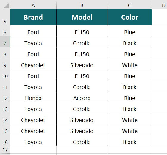
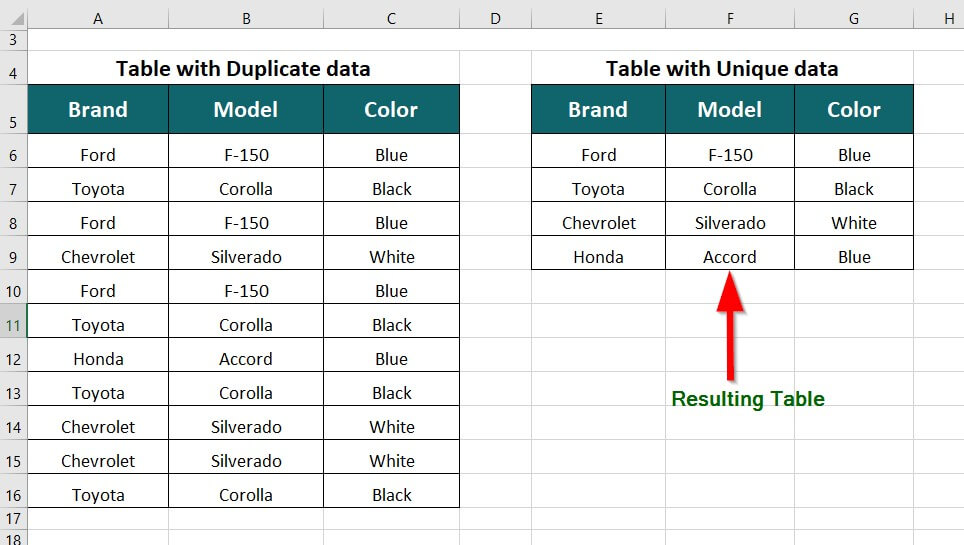
The table below shows the brand name of four-wheelers and their model name and color. Using Excel’s Advanced Filter, we want to remove the duplicate values.
Solution:
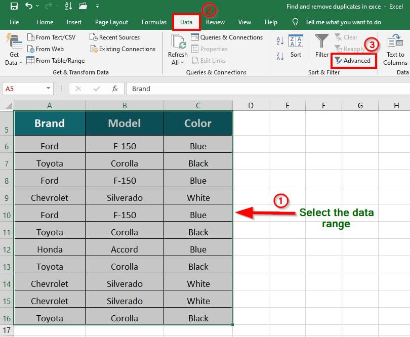
Step 1: Select the data range
Step 2: Go to Data Tab
Step 3: Select the Advanced option under the Sort & Filter Group.
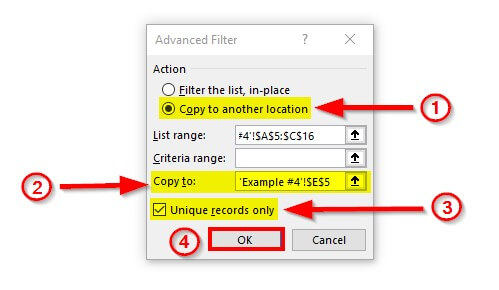
An Advanced Filter dialog box appears
Step 4: Select the Copy to another location option
Step 5: Click the cell in the worksheet where the new(unique) data table needs to be created. This will fill the section Copy to.
Step 6: Click the checkbox Unique records only.
This results in a table with unique data, as shown below
#6 Using the Power Query Tool in Excel to Remove Duplicates
You can integrate data from different sources, clean up your data, and transform it using Excel’s Power Query feature. Duplicates in Excel can be easily removed using this utility.
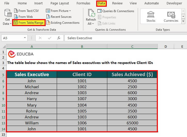
Step 1: Choose a cell or region, then find the Data Tab’s – Get & Transform Data section and click the From Table/Range option.
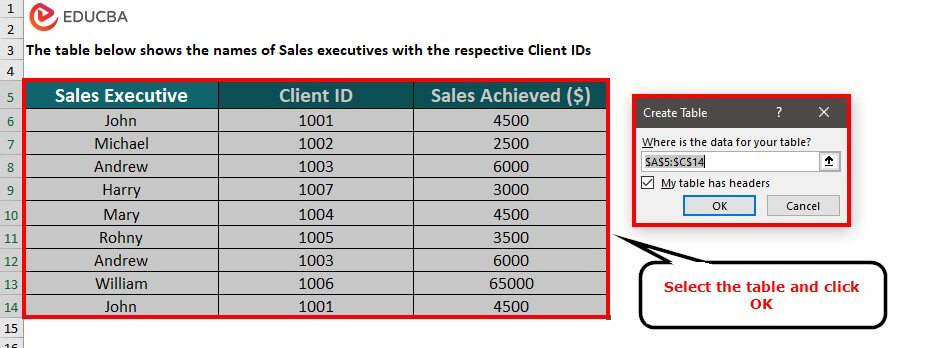
A dialogue window for creating a power query table will appear on clicking.
Step 2: Verify that the stated range of values is accurate.
Step 3: Select OK.
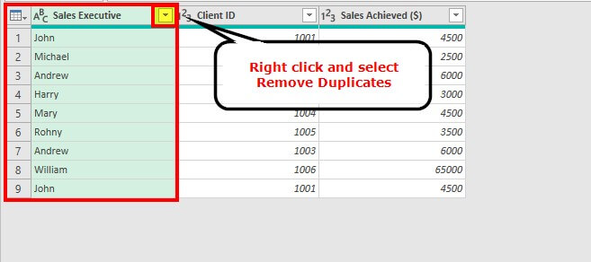
The Power Query editor window opens.
We now have two choices. Based on the following, copies can be eliminated:
- One or more columns
- Entire table
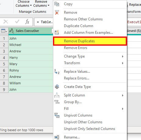
Step 4: Right-click on the relevant ‘column heading’ to delete duplicate entries based on one or more columns. Using the SHIFT button, we can pick multiple columns. In this example, we have selected the Sales Executive column.
Step 5: Select the “Remove Duplicates” choice after that.
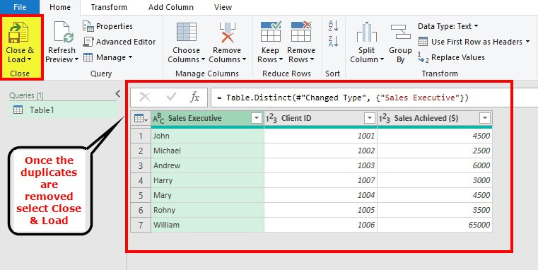
The data will be free of duplicate values in this manner.
Step 6: Clicking the “Close & Load” choice in the upper left corner will load the data onto the spreadsheet.
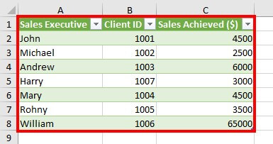
The data will be visible as per the below screenshot.
Things to Remember
- We can remove duplicates from Google Sheets using the Data Cleanup option
- It is important to remove any subtotal before using the feature Remove Duplicates in Excel.
- It is recommended to make a copy of your worksheet before trying to remove duplicate data.
Frequently Asked Questions (FAQs)
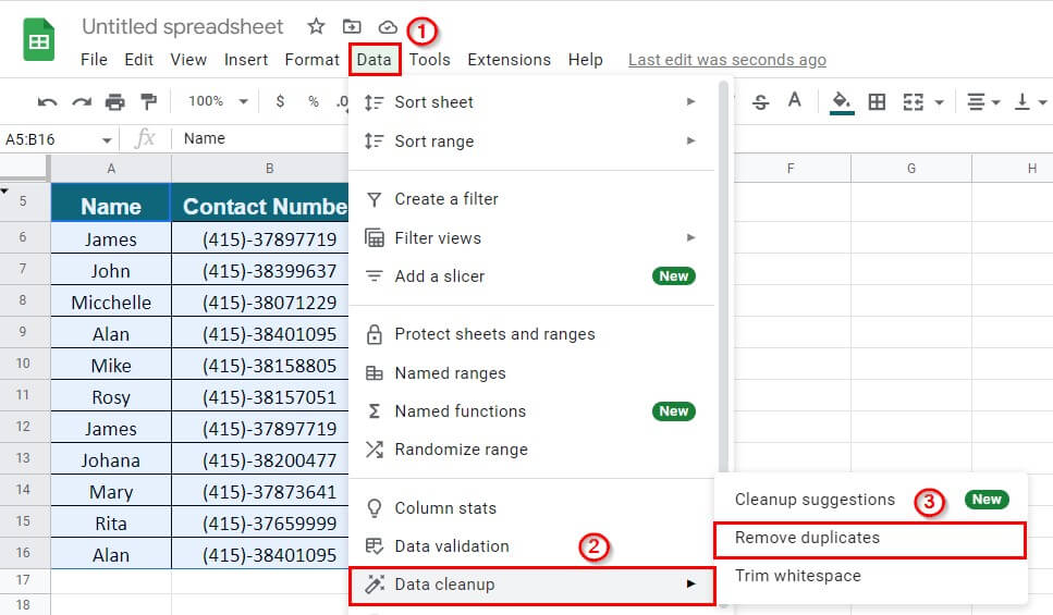
Q1. How do I quickly delete duplicates in Google Sheets?
Answer: To delete duplicates in Google Sheets, follow these steps:
Step 1: Select the data table
Step 2: Go To Data > Data cleanup > Remove duplicates
Q2. Where is the removal of duplicates in Excel?
Answer: To find the Remove Duplicates option in Excel, follow these steps:
Step 1: Go to the Data Tab of the Excel toolbar
Step 2: Under the Data Tools Group, click on the Remove Duplicates icon (option), as shown below
Q3. What is the shortcut to finding duplicates in Excel?
Answer: To find and highlight duplicates in Excel, press the below keys one by one,
ALT + H + L + H + D.
When we press the above keys, the duplicate values (rows) will be highlighted in the provided color. The keys function as a shortcut for the conditional formatting features in Excel.
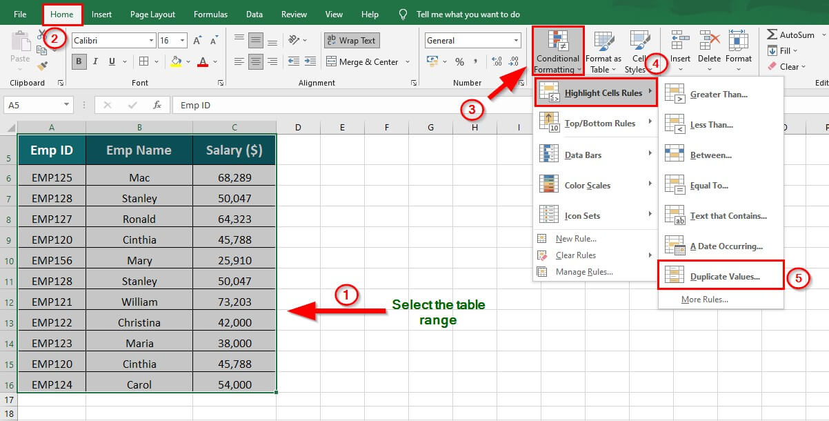
Q4. How do I find and keep only duplicates in Excel?
Answer: To find and keep the duplicate values in Excel, follow the below steps:
Step 1: Select the data table
Step 2: Go to the Home Tab
Step 3: Under the Styles Group, go to,
Conditional Formatting > Highlight Cells Rules > Duplicate Values
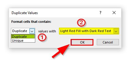
A Duplicate Values dialog box will appear,
Step 4: Select the Duplicate option from the drop-down list and choose the desired highlight color and Click OK
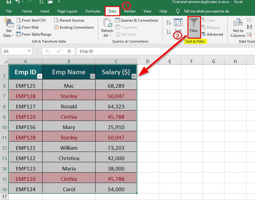
All the duplicate values in the table will be highlighted.
Step 5: Select the data table and go to Data Tab
Step 6: Under the Sort & Filter Group, click on Filter
This will apply a filter to the data set, as shown below
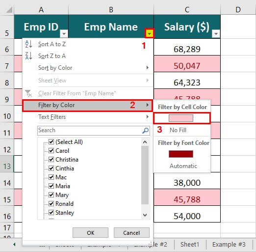
Step 7: Click on the filter icon of column B (Emp Name)
Step 8: Click on Filter by Color
Step 9: Select Filter by Cell Color
The highlighted duplicate values will be filtered as shown below
Recommended Articles
The above article explains how we can find and remove duplicates in Excel worksheets. To learn more about such useful features of Excel, EDUCBA recommends the below-given articles.
