Updated May 3, 2023
REPT Function in Excel
Rept function in Excel returns the text value of any cell or cell range and repeats those text range in a cell with a number of repetition we allow. For example, in 3 selected cells have One, Two and Three as text values, so using Rept function, we can call all the select text values in one cell and repeat them as well more than 1 time if required in the same cell.
REPT Formula in Excel:
The Formula for the REPT Function in Excel is as follows:
Where the supplied arguments are:
- Text – The text you want to repeat.
- Number_times – The number of times to repeat that text.
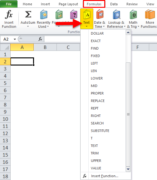
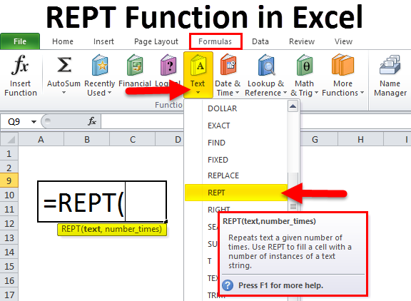
As the REPT function is a built-in function in excel and categorized under the Text/String functions category, thus it’s listed under the FORMULAS tab. Please follow the below steps:
- Click on the FORMULAS tab.
- Select the Text functions category. It will open up a drop-down list.
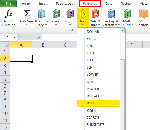
- Click on the REPT function from the listed functions.
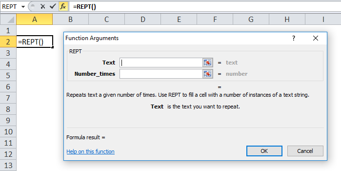
- After clicking on the REPT function, a Function argument box will open up.
- Pass the first argument of the REPT function, which is text. The text which you want to repeat.
- The second argument is Number_times, it specifies the number of times to repeat the text. It is a positive number.
How to Use REP Function in Excel?
REPT Function in Excel is very simple and easy to use. Let’s understand the working of REPT in Excel by Some Examples.
Example #1
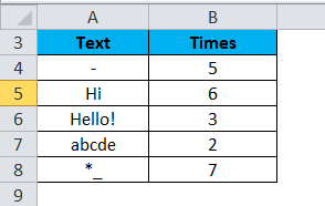
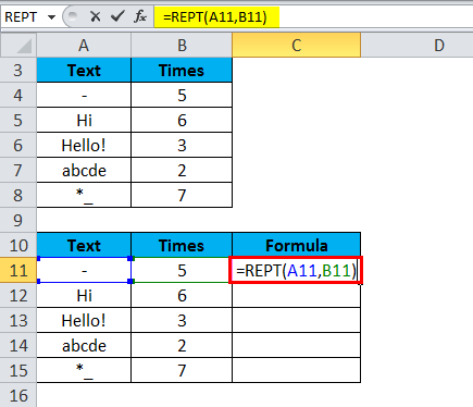
We have given the below data:
Now we will apply the REPT function on the above data:
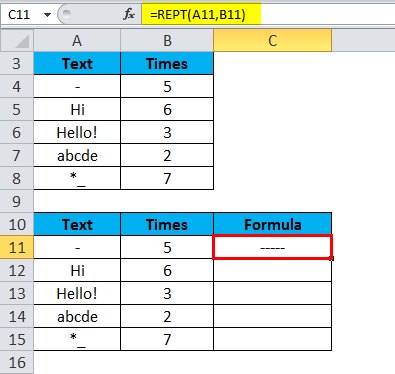
As per the above screenshot, the REPT function will repeat the character “_“ hyphen 5 times.
Now drag & drop this function for the below values.
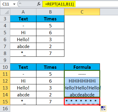
The final result is:
Example #2
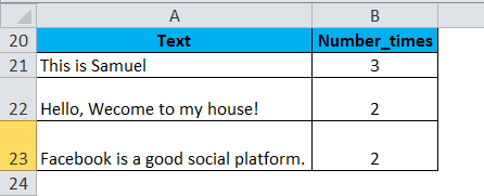
We also can apply the REPT function on a string as well.
We will apply the REPT function here
The results are:
Now drag & drop this function for the below values.
Example #3
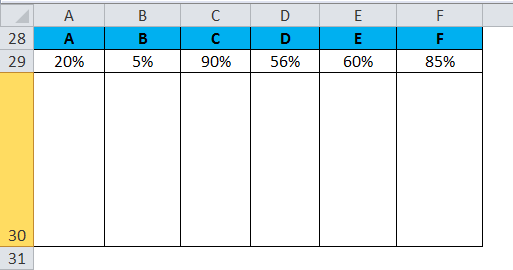
To create a simple in-cell chart or column chart, we will use the REPT function. Here we will use percentage data to create the cell chart.
The steps are as follows:
- Please increase the size/height of the row where you want to insert the chart so that the column bar will adjust in it.
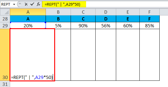
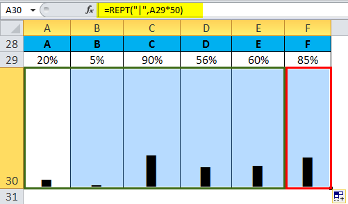
- Insert the REPT function formula in cell A30 and enter.
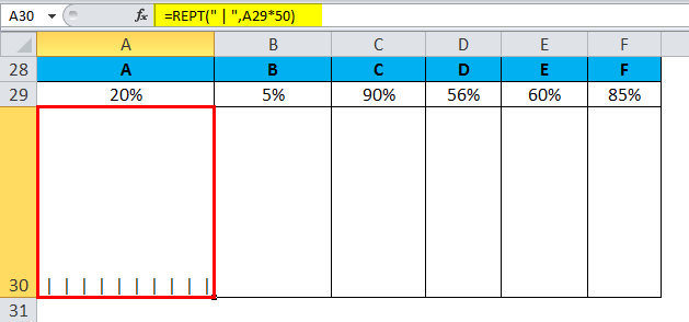
The result is:
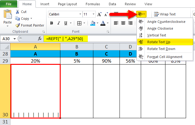
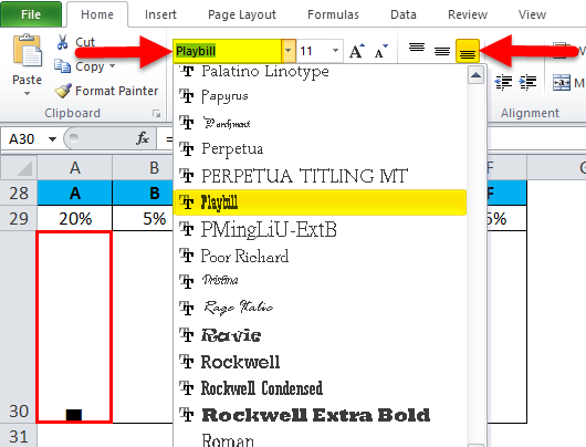
- Now, change the orientation of the text to “Rotate Text Up” as per the below screenshot.
- Change the font style to PLAYBILL and alignment to bottom & center.
- Apply the same steps for the rest values.
- Finally, you will get the In-cell column chart.
With the same steps, you can also create an In cell bar chart too.
Example #4
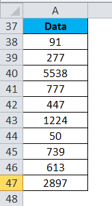
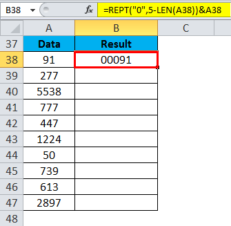
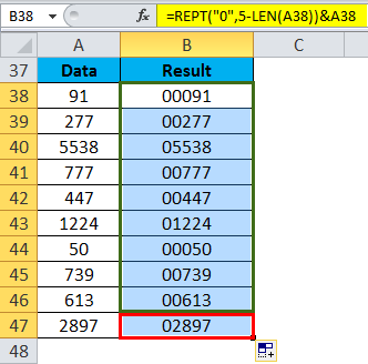
We have given the financial data, and it is needed to make all the numbers of the same length. For this, we will add Zero in the numbers in such a way so that the value of the number doesn’t change.
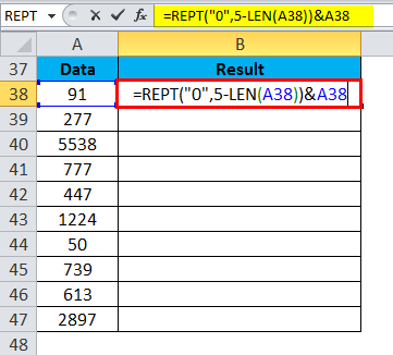
We want all the numbers should be of length 5. For this, we will use the REPT function:
The result is:
Drag & drop the above function for the rest values, and the final results are:
Explanation:
- We will first take the length of the string.
- Then subtract the length from 5 (mentioned length which we want to make for all numbers).
- REPT function will return the number of 0’s based on the number, which occurs after subtracting from the number 5.
For example, If the number is 91, it would return 000.
Things to Remember
- If the second argument number_times is Zero, the function returns an empty string.
- If number_times is a decimal value, it will truncate to an integer. For example, if the values are 5.93, it will only consider 5.
- The result of the REPT function must be no longer than 32,767 characters. Otherwise, it will return #VALUE! error.
Recommended Articles
This has been a guide to REPT in Excel. Here we discuss the REPT Formula in Excel and how to use the REPT Function in Excel along with excel example and downloadable excel templates. You may also look at these useful functions in excel –

