RIGHT Formula in Excel (Table of Contents)
Excel RIGHT Formula
Excel RIGHT function is a built-in function that is categorized under text/string function, which can be used to extract the specified number of substrings from a string starting from the rightmost letter or from the end of your string.
Syntax
An argument in RIGHT Formula
- text – Required argument specifies the text/string or the cell containing the string you wanted to extract the substring from.
- num_chars – This is an optional argument that specifies the number of characters extracted from the given string from the left-hand side or the start of the string.
- If num_chars is omitted, by default value, 1 will be considered, which means the last character of your string will be published as a result.
- If num_chars is greater than the length of your string (or the total number of characters in your string), the RIGHT formula will publish the entire string as an output.
- If num_chars is negative, the RIGHT formula will give the #Value! error.
How to Use RIGHT Formula in Excel?
RIGHT Formula Excel is very simple and easy. Let’s understand how to use the RIGHT Formula in Excel with some examples.
Example #1 – Extract Substring from a String
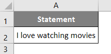
Suppose you have a string as shown in the cell given below.
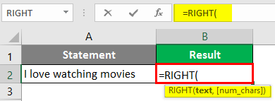
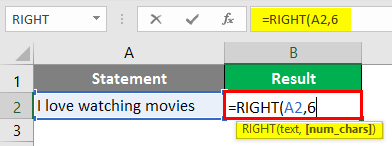
In Cell B1, start typing the formula for the RIGHT formula, as shown below.
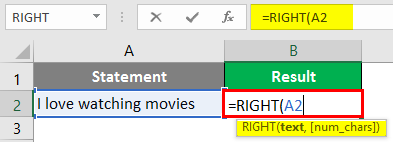
The first argument for the RIGHT function is the text value from which we need to extract the substring. Mention A2 as the first argument for the Right Formula.
Add numeric value 6 as a text specifier, which specifies the number of substrings you want to extract from the main string through the right-hand side.
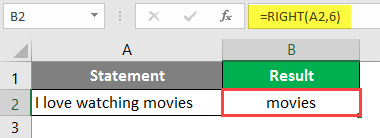
Press Enter Key to see the output. You’ll see the output below.
This is how the Excel Right function can be used. It just simply extracts the substring from the right of your string based on the number of characters argument you specify.
Example #2 – Extract Substring after a Specific Character
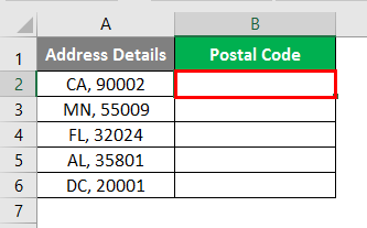
Suppose we have data like the one below, with State Code and Postal Code details.
What if we extract the postal code details from this combined text? We can achieve this result by combining Excel RIGHT, LENTH, and SEARCH functions. Let’s see this step by step.
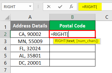
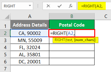
Start typing Excel RIGHT Formula under Cell B2.
It would be best to give the first argument as the string you want to extract the substring. In this case, you can provide A2 as a first argument because it contains the text value from which you want to extract the substring.
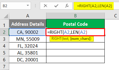
Use the LEN function to get the length of the cell containing the string.
As the function will extract the data from the right, it should know the exact length of the text to search the specific delimiter and return the expected substring.
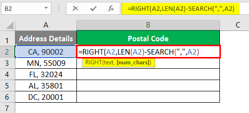
Now, use the SEARCH function to find the specific delimiter in the cell containing text and subtract it from the text length in A2.
Please don’t get confused; it seems confusing to the naked eye. Let us try to evaluate the logic behind this.
- SEARCH function gives the position at which the delimiter value occurs in our cell (3rd position). That position value is subtracted from the total length of cell A2 (the length of cell A2 is 9, which includes 7 character letters, one comma, and one space). So, after subtracting (9 – 3 = 6), we get 6 as a num_chars argument of the RIGHT function. Thus, the RIGHT function extracts 6 characters from the right of the string.
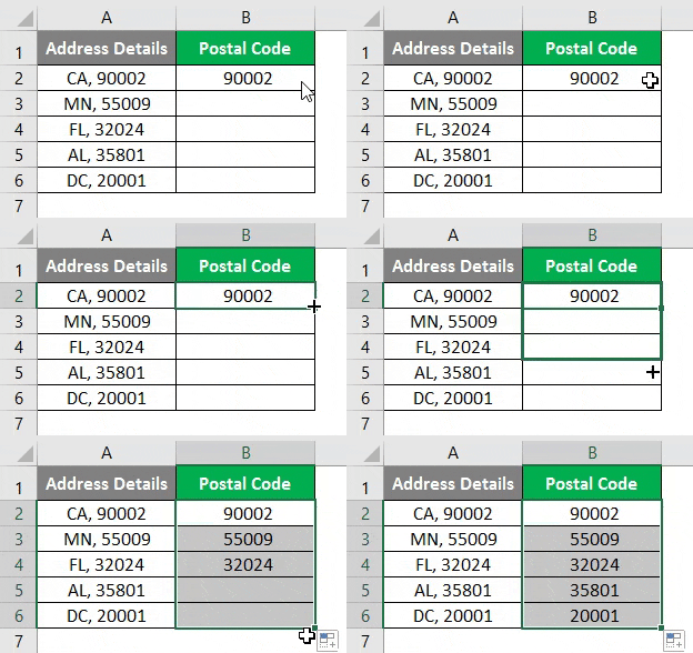
Press Enter Key and drag the formula to row B6 to see the output of this formula.
One obvious question arises: why can’t we directly provide the num_chars argument in this formula? The reason is that the delimiter would not be at exactly the same position every time. Sometimes, it might be a different position (for example, in the case of full name). It would be difficult to provide the num_chars argument manually every time. Therefore we better automate things using formulas.
Example #3 – Store the Number Values Only
As discussed at the start of this article, the RIGHT formula is categorized under the text formula in Excel. If you extract any numerical value, it will be stored as text. However, you might need to get those values as numbers only. Let’s see how we can do this.
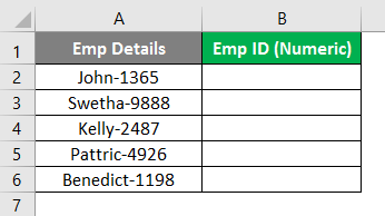
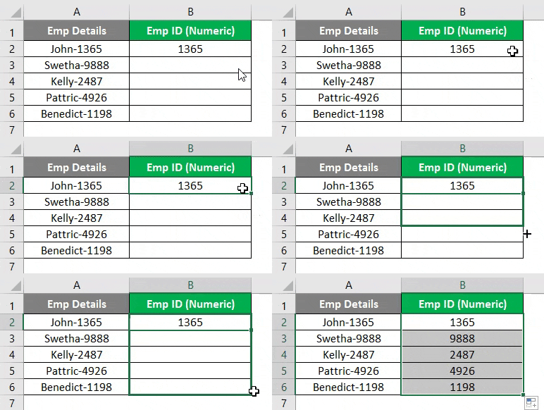
Suppose we have data containing the employee’s first name and the employee code, which is a numeric value. We must store this employee code as a number for further data calculations.
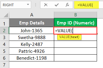
Start typing VALUE Formula in Cell B2 (We do this so that the value we extract can be stored as a number in Excel).
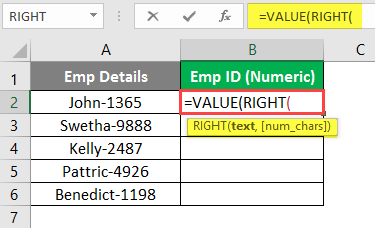
Use Excel RIGHT as an argument under the VALUE function. It will take that formula as an argument because the RIGHT formula is for text manipulation, and the VALUE function can convert a text value into a numerical value.
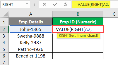
Give A2 as an argument to the RIGHT formula, as it contains the string we need to extract the substring.
You can see that the employee ID is of length 4 from the right-hand side of the string for all the cells (It can also be manipulated using the LEN-SEARCH formula as we did in the previous example). Therefore, use 4 as a num_chars argument.
Press Enter Key and Drag the Formula till Cell B6 to see the output.
You can see the output in the screenshot above. We align the values from Cell B2 to B6 in column B. Therefore, you can say that those are being converted into numbers.
This is it from the article. Let’s conclude by highlighting some key points to remember.
Things to Remember About RIGHT Formula in Excel
- The default value for the num_chars argument is 1. It extracts the first character string from the right of the string.
- The num_chars value should always be greater than or equal to 1. If it’s less than 1 (or negative in that case), it gives #VALUE! Error.
- If the num_chars value exceeds the length of the entire string, the RIGHT formula gives an entire string as an output.
Recommended Articles
This is a guide to RIGHT Formula in Excel. Here we discuss How to use RIGHT Formula in Excel, practical examples, and a downloadable Excel template. You can also go through our other suggested articles –
