Updated May 9, 2023

Introduction to ROUND Formula in Excel

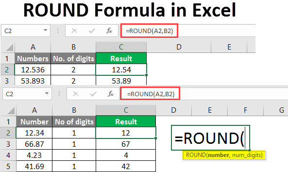
The ROUND Formula in Excel returns the rounded value of a supplied number to a specified number of decimal places. In simple terms, this function rounds off a number to a given number of digits. This function is present in all versions of MS Excel. The Round function in Excel falls under the “Math & Trigonometry” formulas. This function can be used as a worksheet function.

Syntax:

Arguments:

Number: The number that we want to round.
No. of digits: This is the number value. It is the number of digits of the decimal place we want our number to round off.

How to Use ROUND Formula in Excel?

We will learn how to use the function and how this will make the calculation of numbers or currency easier. Here are some examples.

You can download this ROUND Formula Excel Template here – ROUND Formula Excel Template

Example #1 – Round Off a Number

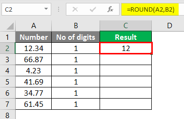
Here we want to round off a number to 1 digit. So we use the ROUND Formula in cell C2.

After using this formula, the answer is shown below.

Drag the same formula in cell C2 to cell C7.

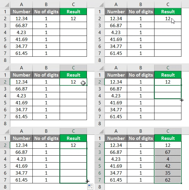
Here the function will round off the number to one digit to the right of the decimal. The numbers above 5 will be rounded up, and those below 5 will be unchanged.

Example #2 – Finding the Rounded Number

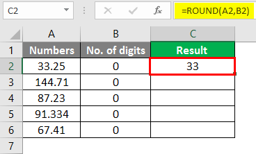
To find out the rounded number when the number of digits is 0. We will use the ROUND Formula in Cell C2.

After using this formula, the answer is shown below.

Drag the same formula from cell C2 to cell C7.

We have some numbers below, and we will see how the number is rounded off when we have 0 as the of digits. The numbers are rounded off to the nearest integer when the number of digits is 0.

As shown above, the number 33.25 is rounded to 33, 144.71 is rounded to 145, and the first digit after the decimal is 7. And so other remaining numbers will be rounded to the nearest whole number.

Example #3 – Using the ROUND Formula

If the number of the digits is 2, the numbers will be rounded off, as shown below. We are using the ROUND Formula in Cell C2.

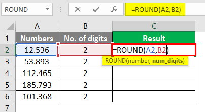
After using this formula, the answer is shown below.

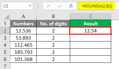
We have a table of numbers that we want to round off up to 2 decimal places. Drag the same formula in cell C2 to cell C6.

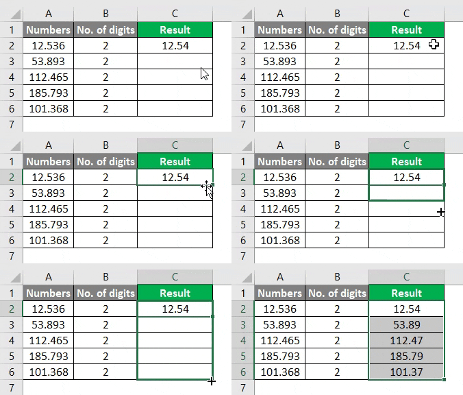
Here the number is rounded to two decimal places. For 12.539 is rounded off to 12.54, and the number 112.465 is rounded off to 112.47 as the last digit after the decimal is 5 or greater than 5, thus rounding off the previous digit.

Example #4 – Rounding Off to Nearest Value

When we have -1 as the number of digits, the number will be rounded off as below. We are using the ROUND Formula in cell C2.

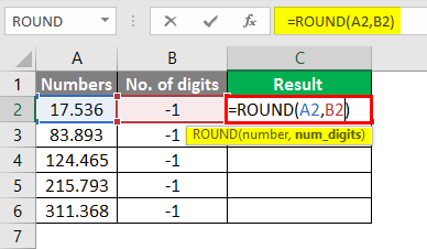
After using this formula, the answer is shown below.

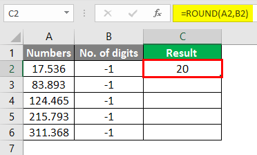
Drag the same formula from cell C2 to cell C6.

The numbers will be rounded to the nearest 10th value when it is a -1 place of decimal. 17.536 is rounded off to 20, 83.893 is rounded off to 80, and so 124. 465, 215.793 and 311.368

They are rounded off to their nearest 10th, respectively.

Example #5 – Rounding the Negative Number

How is the negative number rounded when the number of digits is 1? We will see this in the below table. We are using the ROUND Formula in cell C2.

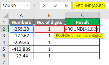
After using this formula, the answer is shown below.

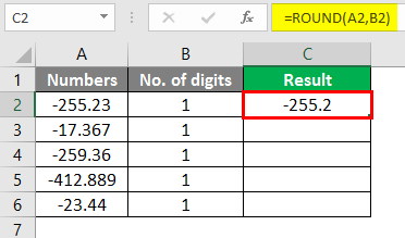
Drag the same formula in cells C2 to C6.

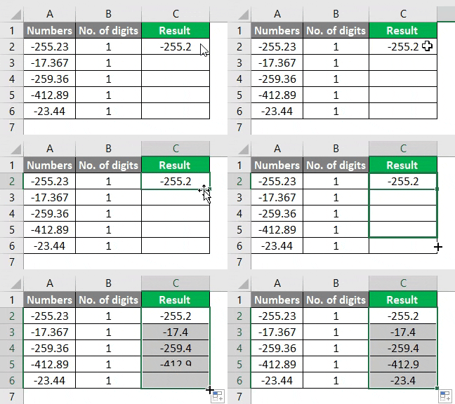
The rounded numbers are easy to calculate. Here the numbers are rounded off to one place of decimal as it would have been in a positive number. These were some examples of the ROUND function in Excel showing how the number is rounded off depending on the number of digits.

Here is an example showing how rounding numbers works in the calculation.

Example #6 – Calculate Commission Sales

Here we have a sample data table showing sales executives’ sales, and we have to calculate the commission on those sales.

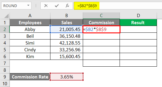
After using this formula, the answer is shown below.

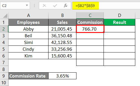
In cell C7, we are using the SUM Formula.

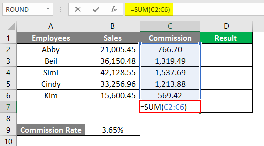
After using this formula, the answer is shown below.

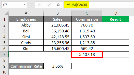
In cell C2, we are using the ROUND Formula.

After using this formula, the answer is shown below.

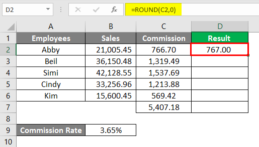
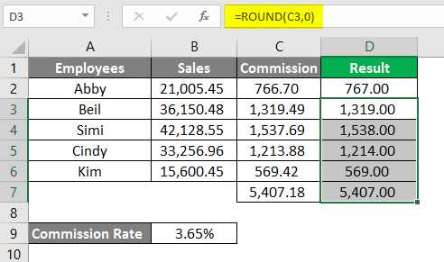
In the above example, the commission is calculated to 2 decimal places. When we rounded the values to 0, the values became rounded and were easy to understand and could be easily communicated.

Example #7 – Rounding off the Numbers by Cell Formatting

We can also round off a number by changing the cell format. You can do this in the below steps:

Select a cell containing the number that you want to round off.
Press CTRL+1 to open the format cell dialog box, go to the number or currency tab, and then type in the number of decimals you want to see in the decimal box.
Click Ok and close the dialog box.

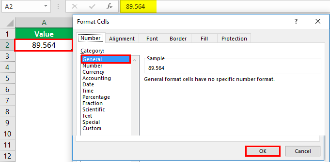
Then,

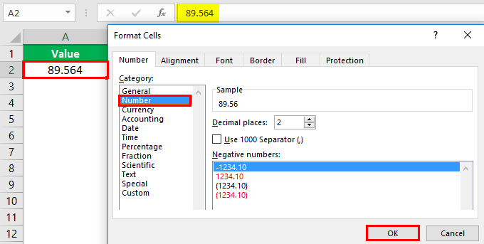
Select the decimal places.

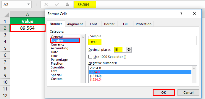
Press the OK Key. You will see the number rounded off below.

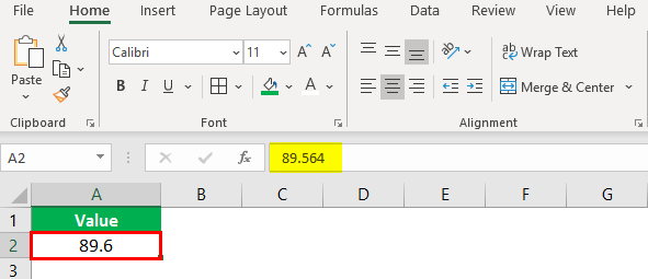
This is also an alternative method for rounding off numbers.

Also there are two other forms of ROUND functions:

ROUNDUP – This function rounds the number upward per the specified number of digits.
ROUNDDOWN – This function rounds the number downwards per the specified number of digits.

Going through the above examples, you will be able to understand the ROUND function and its uses in Excel. It is a commonly used function in calculations and the presentation of numeric data.

Things to Remember About ROUND Formula in Excel

The ROUND function comes under the Math and Trigonometry function.
The function rounds off a number as per the number of digits specified.
There are some cases where ROUNDUP and ROUNDDOWN functions suit better than the ROUND function.
When the number of digits is from 1-4 after the decimal, the ROUND function will round the number down. And when the digit is from 5-9, the function will round up the number.
If the number of digits is greater than 0, the number is rounded to a specified number of digits to the right of the decimal point.
When the number of digits is less than 0, the number is rounded to a specified number to the left of the decimal point.
If the number of digits equals 0, the number is rounded to the nearest whole number.