Updated August 16, 2023
Excel Rows to Columns (Table of Contents)
Rows to Columns in Excel
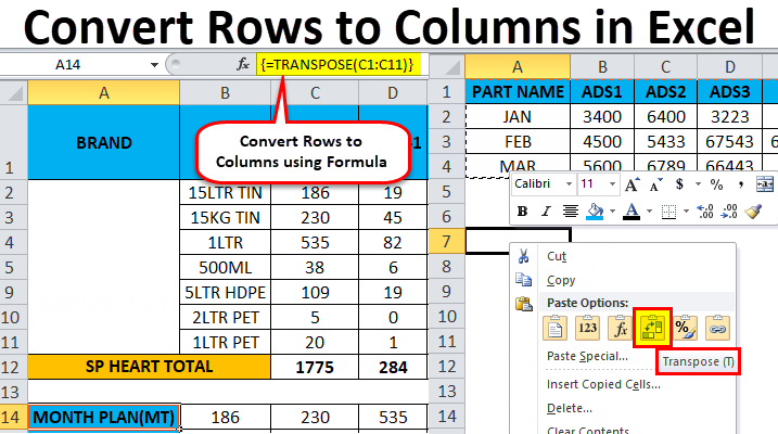
In Microsoft Excel, we can change the rows to columns and columns to rows and vice versa, using TRANSPOSE. We can either use the Transpose or Transpose function to get the output.
Definition of Transpose
The transpose function normally returns a transposed range of cells which is used to switch the rows to columns and columns to rows and vice versa, i.e., we can convert a vertical range of cells to a horizontal range of cells or a horizontal range of cells to a vertical range of cells in Excel.
For example, a horizontal range of cells is returned if a vertical range is entered, or a vertical range of cells is returned if a horizontal range of cells is entered.
How to Convert Rows to Columns in Excel using Transpose?
It is very simple and easy. Let’s understand how to convert rows to columns in Excel using examples.
Steps to use transpose:
- Start the cell by selecting and copying an entire range of data.
- Click on the new location.
- Right-click the cell.
- Choose to paste special, and we will find the transpose button.
- Click on the 4th option.
- We will get the result converted to rows to columns.
Example #1
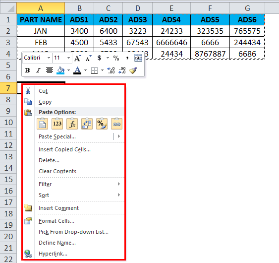
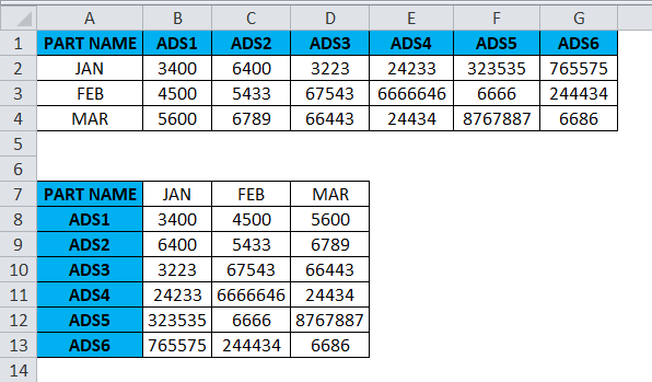
Consider the below example where we have a revenue figure for sales month-wise. We can see that month data are row-wise and Part number data are column-wise.
If we want to convert the rows to columns in Excel, we can use the transpose function and apply it by following the below steps.
- First, select the entire cells from A To G with data information.
- Copy the entire data by pressing the Ctrl+ C Key.
- Now select the new cells where exactly you need to have the data.
- Right, click on the new cell, and we will get the option shown below.
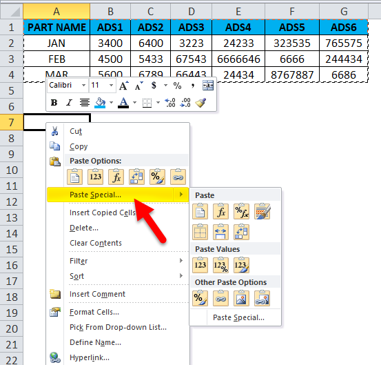
- Choose the option paste special.
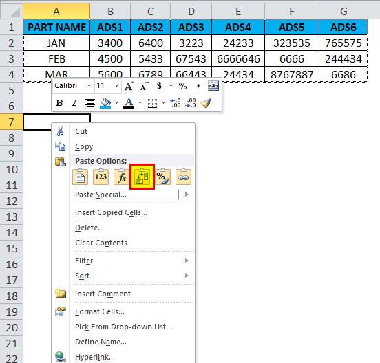
- Select the fourth option in paste special, transpose, as shown in the below screenshot, highlighted in yellow.
- Once we click on transpose, we will get the following output.
In the above screenshot, we can see that rows have been changed to the column, and the column has been changed to rows in Excel. This way, we can easily convert the given data from row to column and column to row in Excel. For the end-user, if there is a huge amount of data, this transpose will be very useful, and it saves a lot of time instead of typing it, and we can avoid duplication.
Example #2
In this example, we will convert rows to columns in Excel and see how to transpose the employee salary data by following the steps below.
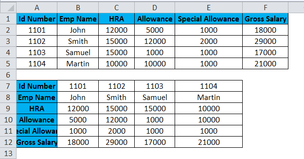
Consider the above screenshot, which has the id number, emp name, HRA, Allowance, and Special Allowance. Suppose we need to convert the data column to rows; in these cases, the TRANSPOSE function will be very useful to convert it, which saves time instead of entering the data. We will see how to convert the column to a row with the below steps.
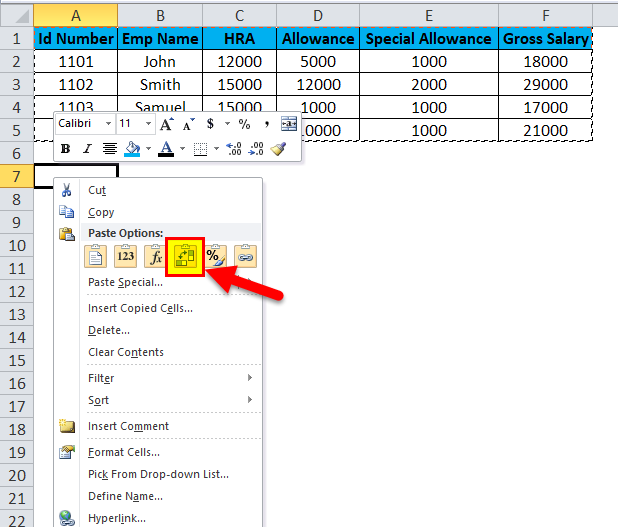
- Click on the cell and copy the entire range of data as shown below.
- Once you copy the data, choose the new cell location.
- Right-click on the cell.
- We will get the paste special dialogue box.
- Choose the Special Paste option.
- Select the Transpose option in that, as shown below.
- Once you have chosen the transpose option, the Excel row data will be converted to the column, as shown in the below result.
In the above screenshot, we can see the difference that the row has been converted to columns; in this way, we can easily use the transpose to convert horizontal to vertical and vertical to horizontal in Excel.
Transpose Function
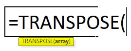
In Excel, a built-in function called Transpose Function converts rows to columns and vice versa; this function works like transpose. i.e., we can convert rows to columns or columns into rows and vice versa.
Syntax of Transpose Function:
Argument
- Array: The range of cells to transpose.
When a set of an array is transposed, the first row is used as the first column of an array, and in the same way, the second row is used as the second column of a new one, and the third row is used as the third column of the array.
If we use the transpose function formula as an array, we have CTRL+SHIFT +ENTER to apply it.
Example #3
In this example, we will see how to use the transpose function with an array with the example below.
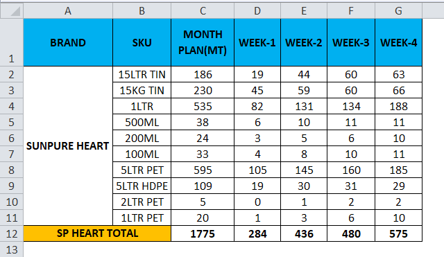
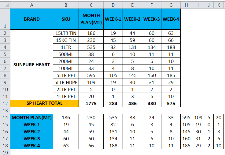
Consider the below example, which shows weekly sales data, where we will convert the data to columns to row and row to column and vice versa using the transpose function.
- Click on the new cell.
- Select the row you want to transpose.
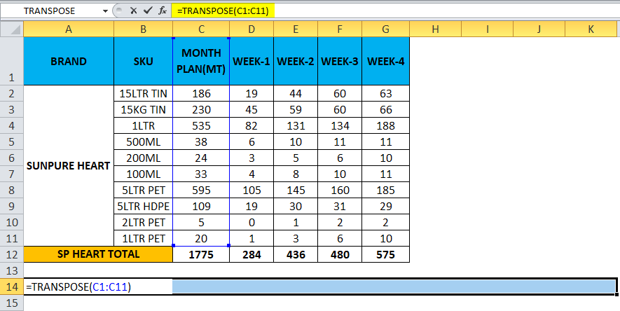
- Here we are going to convert the MONTH PLAN to the column.
- We can see that there are 11 rows, so to use the transpose function, the rows and columns should be in equal cells; if we have 11 rows, then the transpose function needs the same 11 columns to convert it.
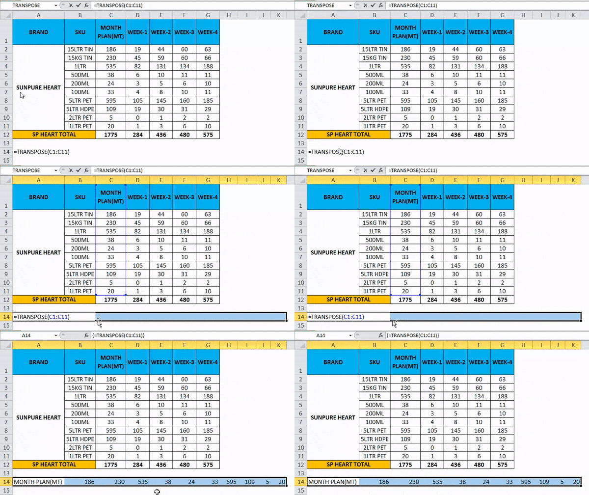
- Choose exactly 11 columns, use the Transpose Formula, and select an array from C1 to C11, as shown in the below screenshot.
- Now use CTRL+SHIFT +ENTER to apply as an array formula.
- Once we use the CTRL+SHIFT +ENTER, we can see the open and close parenthesis in the formulation.
- We will get the output where a row has been changed to a column, shown below.
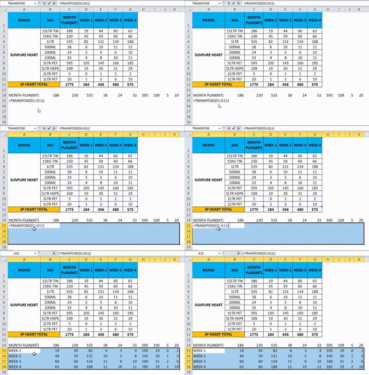
- Use the formula for the entire cells to get the exact result.
So the Final Output will be as below.
Things to Remember About Convert Rows to Columns in Excel
- The transpose function in Excel is one of the most useful functions, as it allows us to rotate the data without altering its information.
- If any blank or empty cells exist, transpose will not work, giving the result zero.
- While using the array formula in the transpose function, we cannot delete or edit the cells because all the data are connected with links, and Excel will throw an error message that “YOU CAN NOT CHANGE PART OF AN ARRAY.”
Recommended Articles
This has been a guide to Rows to Columns in Excel. We discuss converting rows to columns in Excel using transpose, practical examples, and a downloadable Excel template. Transpose can help everyone to convert multiple rows to a column in Excel easily and quickly. You can also go through our other suggested articles –
