What is the Search Formula in Excel?

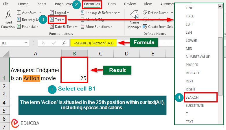
The SEARCH formula in Excel tells us the position at which the first character of a particular text appears in a cell or a text string.

If we have the text “Hello, how are you?” in a cell and use the SEARCH function to find the position of “how,” the result will be 8. This is because “how” begins at the eighth position in the text (considering the comma and space too).

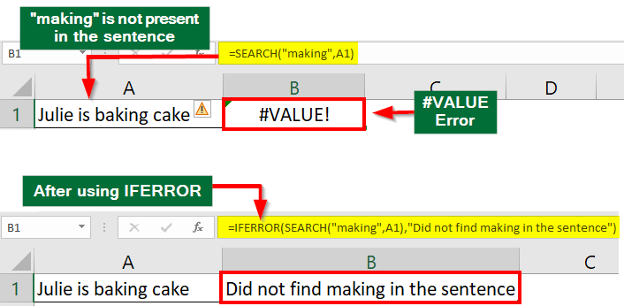
Remember that if the formula does not find the substring, it returns a #VALUE! Error.

What is the Search Formula in Excel?
Syntax & Arguments
How to Use Search Formula in Excel?
Examples of SEARCH Formula in Excel
SEARCH Vs. FIND Formula
Using Search with Other Functions
Things to Remember

Syntax

Arguments

find_text: This is the substring you want to find within the within_text string.
within_text: This is the text string where you want to search for the find_text.
start_num (optional): This argument specifies the starting position of the search within the within_text. If not provided, the search starts from the beginning of the within_text.

How to Use Search Formula in Excel?

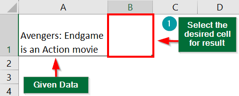
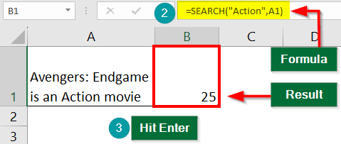
1. Open your Excel spreadsheet and select the cell where you want the result to appear.
2. Type the formula =SEARCH(“Action”,A1)

3. Press Enter.

Examples of SEARCH Formula in Excel

You can download this SEARCH Formula Excel Template here – SEARCH Formula Excel Template

#1: How to Search a Single Character in a Word?

Suppose you want to find the position of the letter “c” in the word “Barcelona.” To do this, follow these steps,

Choose a cell where you want the search result to appear. Let’s say you choose cell B1.
In Cell B1, type =SEARCH(“c”, A1)
Press the Enter

Result:
Cell B1 will now display the position of the character “c” in the word “Barcelona” as 4.

#2: How to Search a Single Word in a Sentence?

If you want to locate the position of the word “whispers” within the sentence “Stars are the whispers of ancient light.” you can follow the below-given steps,

Choose the desired cell for the result, i.e., cell B1.
In cell B1, type the following formula: =SEARCH(“whispers”, A1)
Press Enter

Result:
The cell will now display the position of the word “whispers” within the sentence as 15. This will also include the spacing between the words.

#3: How to Search First Space in a Sentence?

Let us see how to find the position when the first space appears in the sentence – “Joey doesn’t share food!”.

Select cell B1 for the result.
In selected cell, enter the formula: =SEARCH(” “, A1)
Press Enter

Result:
The function will return the position of the first space as 5.

#4: How to Use SEARCH on a Range of Cells?

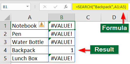
You have a list of school items, and you want to search the cell that contains the word “Backpack”.

Choose a cell for the result (E.g., cell B1).
Enter =SEARCH(“Backpack “, A1:A5)
Press Enter

Result:
The formula searches for the text “Backpack “within each cell in the range A1: A5. It finds “Backpack ” in cell B4 and returns the result as 1. It displays an error message for all other cells because it did not find the word in those cells.

#5: How to Search Using start_num?

Suppose you have the following sentence: “I enjoy reading both classic novels and classic poetries.” Here, the word “classic” appears twice. Now, if you want to find the starting position of the second occurrence of the word “classic,” you can use the “start_num” option.

1. Enter the formula without the “start_num” argument like this: =SEARCH(“classic”, A1) and press enter. You will get the result as 22.

2. Now, to find the second instance of the word, just add 1 to 22 (22+1 = 23) and then use that number (23) as the “start_num” argument.
3. The formula will be: =SEARCH(“classic”,A1,23). Now enter this in the result cell.
4. Finally, press the Enter

Result:
The resulting cell shows the position of the second “classic” as 41.

Note: The SEARCH formula in Excel starts searching for the word “classic” after the 23rd position in the sentence. This way, it passes the first occurrence of “classic” and can find the second occurrence.

#6: How to Use Nested SEARCH?

Suppose you want to find the third occurrence of a specific character or word. If you follow the steps shown in the previous section, it can be time-consuming. In such cases, we can use nested SEARCH.

Let’s say you have a code “KD-25H-SPD-114” and want to know where the third hyphen appears in this code.

Choose the cell for the result. For our example, it is cell B1.
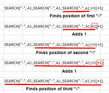
Type =SEARCH(“-“,A1,SEARCH(“-“,A1,SEARCH(“-“,A1)+1)+1)
Press Enter

Result:
Cell B1 displays the position of the third “-” as 11.

The image below explains how the nested SEARCH formula in Excel works:

SEARCH Formula Vs. FIND Formula

In Excel, both the FIND and SEARCH functions help us locate a specific text within a larger text string. However, they differ in how they handle certain aspects of the search.

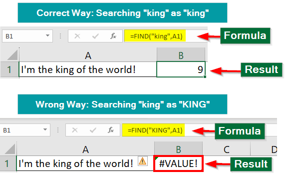
The FIND function is case-sensitive, which means it will only find an exact match of the specified text. The function will return an error (#VALUE!) if the characters don’t match. For instance, if you are searching for “king” using the FIND function, it will only find “king” and not “King” or “KING.”

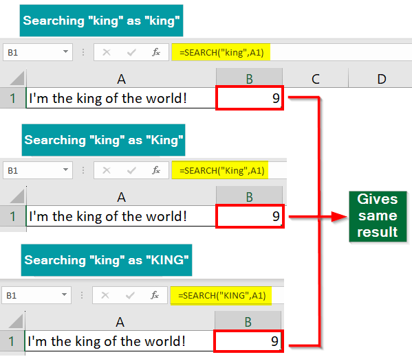
On the other hand, the SEARCH function is not case-sensitive, meaning it will find a match regardless of the case of the characters. So, using the same example, if you are searching for “king” using the SEARCH function, it will find “king,” “King,” and “KING” within the target string.

Advanced Application with SEARCH Formula

1. SEARCH with LEFT Function

We have an order code: “1094 Chair” where “1094” is the order ID and “Chair” is the product. We want to find just the ID.

Solution:
To achieve this, you can employ the SEARCH function along with LEFT:
=LEFT(A2,SEARCH(“ “,A2)-1)

Here’s how this formula works:

The formula starts by searching for the position of the space character within the text “1094 Chair.” The space is in the 5th position.
It then takes the characters to the left of the space.
For the example “1094 Chair,” the space is at position 5. So, it takes characters 1 to 4 (position 5 minus 1) from the text.
The result is “1094,” which is the first part of the original text before the space.

Result:
By applying the formula, you obtain “1094” as demonstrated below:

2. SEARCH with MID

We want to extract the middle name “David” from the full name “Emily David Moore.”

Solution:
Let us use the functions SEARCH and MID. Note that you must know the exact number of characters in the word you are looking for.
=MID(A2,SEARCH(“ “,A2)+1,5)

Here’s how this formula works:

The SEARCH function finds the position of the space in “Emily David Moore.” It’s in 6th position.
The MID function then extracts text from the 7th position onward (space’s position + 1).
The extraction includes 5 characters covering the middle name “David.”
As a result, the formula gives “David” as the extracted middle name from the full name.

Result:
The functions return the middle name correctly as “David.”

3. SEARCH with REPLACE

Suppose you want to change a sentence from “The sun rose over the mountains” to “The moon rose over the mountains” using Excel.

Solution:
To do this, use the SEARCH and REPLACE formulas together.
=REPLACE(A1,SEARCH(“sun”,A1),3,”moon”)

Result:
Excel will return the new statement: “The moon rose over the mountains.”

4. SEARCH with ISNUMBER

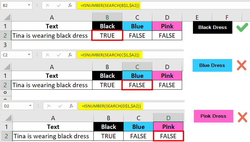
You have a text in cell A2 as “Tina is wearing a black dress.” In cells B2, C2, and D2, you have the colors Black, Blue, and Pink, respectively. Let us determine the color of the dress Tina is wearing.

Solution:
Use the SEARCH formula in Excel with the ISNUMBER function

For searching “Black” in the sentence:

=ISNUMBER(SEARCH(B$1,$A2))

For searching “Blue” in the sentence:

=ISNUMBER(SEARCH(C$1,$A2))

For searching “Pink” in the sentence:

=ISNUMBER(SEARCH(D$1,$A2))

Note: The formulas will give the right answer without the “$” too. However, using the “$” symbol can be beneficial when working with large data.

Result:
If the function locates the given word in the sentence, it shows TRUE instead of the position. If it doesn’t find the word, it shows FALSE instead of an error message #VALUE!

Things to Remember

Case Insensitive: SEARCH() is not case-sensitive, meaning it treats uppercase and lowercase letters the same.
Error Handling: To handle the #VALUE! Error, use the IFERROR function or the IF function combined with the ISNUMBER function.
Cell References: Instead of directly mentioning the data in find_text and within_text, you can also use cell references. For example, if A1 has the word you want to search for and B1 has the main sentence, you can write = SEARCH(A1,B1).
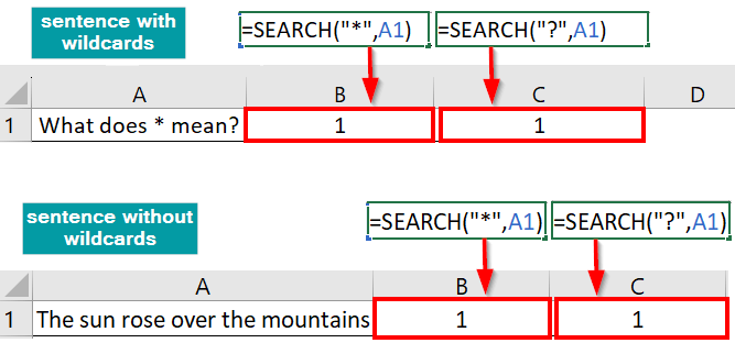
Wildcards: In the SEARCH function, you cannot use the wildcard characters like “*” or “?” for pattern matching. Using these in a SEARCH always gives a result of 1, whether the wildcard is there or not in the sentence.

Frequently Asked Questions (FAQs)

Q1. How can I handle errors when using the SEARCH function?
Answer: Most search functions return error values if they can’t find a match. You can use the IFERROR function to handle the errors in such cases. The IFERROR function will display custom messages or values instead.

Q2. Can I use the SEARCH function to find the nth occurrence of a substring?
Answer: Yes, it is possible to find the nth occurrence of a substring using the SEARCH function. For that, we can use the nested SEARCH function. For a quick recap, check the 6th example of this article.

However, finding the position beyond the 4th occurrence will complicate the formula. In such cases, we recommend using other Excel functions or the method shown in example 5.

Q3. Can we combine the SEARCH formula in Excel with other functions?
Answer: Yes, you can easily use the SEARCH function in combination with functions like IF, LEN, LEFT, RIGHT, etc., to perform more advanced text manipulation and analysis.

Quiz Result
Total Questions	Correct Answers	Wrong Answers	Percentage