Updated June 23, 2023
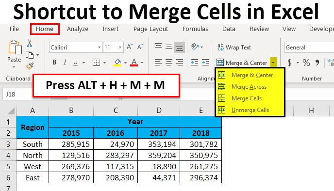
Excel Shortcut For Merge Cells (Table of Contents)
- Shortcut Keys to Merge Cells in Excel
- How to Use Shortcut Keys to Merge Cells in Excel?
- Different Alignment Options
- Limitations of Merged Cells
- Unmerge Cell by Using Excel Short Cut Key
Shortcut Keys to Merge Cells in Excel
When it comes to Excel, creating clear and visually appealing tables is important. One way to achieve this is using the Excel merge cell command. With the Merge Cells command, you can combine neighboring cells into a larger cell, resulting in an easier-to-read table.
It’s particularly useful for creating headers or titles, formatting tables, or improving the visual appearance of your spreadsheet. Merging cells can also center text within the larger cell and apply formatting options like borders and shading, making your table more visually appealing.
Multiple ways to merge cells in Excel include various shortcuts and built-in commands. These methods save time and improve productivity, especially if you need to merge cells frequently. This article will explore some of these shortcuts in detail with step-by-step instructions.
How to Use Shortcut Keys to Merge Cells in Excel?
Example #1
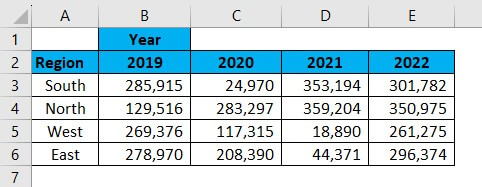
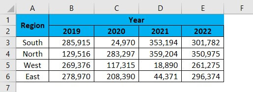
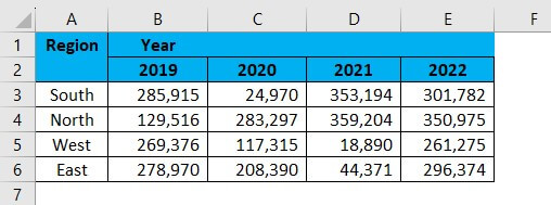
Below is the final sales report that shows sales data organized by year, sales manager, and region. Under the main heading of “YEAR”, each year is listed as a subheading. To improve the visual appeal of the report, we need to merge the “YEAR” cell with the adjacent cells.
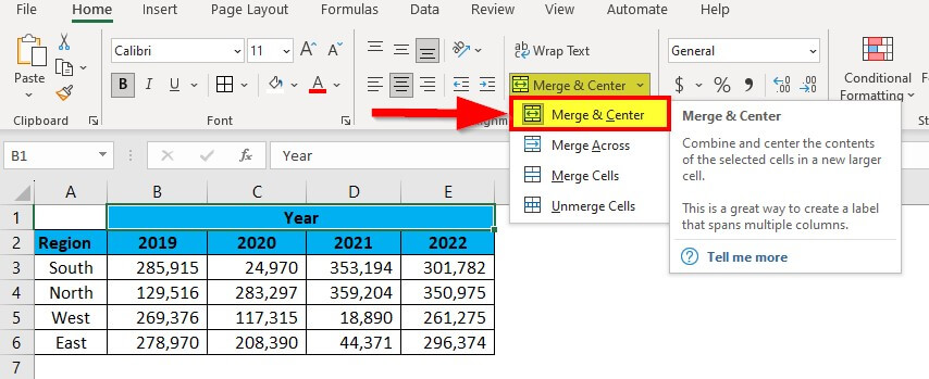
Step 1: Select the number of cells you want to merge. In this example, we want to merge the cells containing the “YEAR” main heading from B1 to E1. To do this quickly, press the shortcut key ALT + H + M + M.
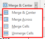
Alternatively, you can use the “Merge & Center” button under the Home tab.
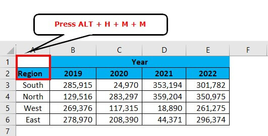
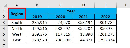
Step 2: Next, we also need to merge the cells containing the region names. To do this, select cells A1:A2 and use the same shortcut key ALT + H + M + M.
This will merge the two cells into one. With the merged cells, the report looks much neater and easier to read.
Example #2
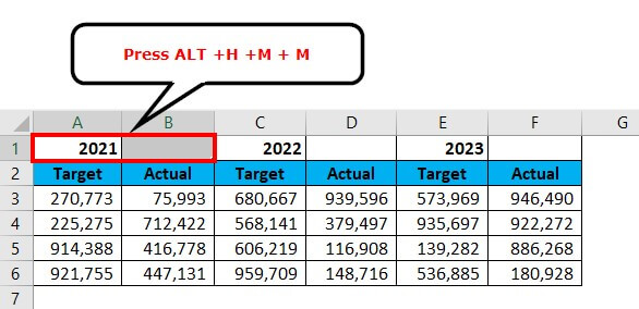
Below is the data for “Target” and Actual numbers for 2021, 2022, and 2023. Let’s see how we can merge the cells for each year and display the Target and Actual data below the corresponding year.
Step 1: Select the cells A1:B1. Press the shortcut key ALT + H + M + M.
It will merge the selected cells.
Step 2: You don’t have to use the merge function for all the remaining years. Rather, simply select the next year and press the F4 function key to repeat the previous action. It will recall the previous action performed.
The final report should look like the below one.
Different Alignment Options
Under alignment, we have different alignment options. Wrap Text, left alignment, right alignment.
Under the “merge & center” function, there are four options.
1. Merge & Centre: This will merge the cells and make the alignment center.
2. Merge Across This will merge the cell and make alignment left alignment.
3. Merge Cells: This will also merge the cell and make alignment left alignment.
4. Unmerge Cells: This will remove all the merged cells to make the value allocated to one cell.
Limitations of Merged Cells
Limitation 1: Selecting a single row using the shortcut key in merged areas is impossible.
Look at the below final report layout.
We cannot use the shortcut key to select one particular row in this merged area. The Ctrl + Space shortcut does not work because it selects all the columns in the merged area, including the unnecessary data.
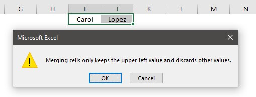
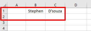
Limitation 2: If we want to merge the first name and last together, it will take out the right-hand side of the data and retain only the left side.
Unmerge Cell by Using Excel Shortcut Key
Just like how we can merge cells, we can also unmerge them. To unmerge a specific portion of the worksheet, we need to first select that portion. And if we want to unmerge all the merged cells in the worksheet, we can simply select the entire worksheet and press ALT + H + M + U.
This will unmerge all the merged cells.
Advanced Techniques for Merging Cells
Merging cells in Excel is a basic technique that can help to organize and present the data in a more readable format. However, some advanced techniques for merging cells can also create more complex spreadsheets. Here are some advanced techniques for merging cells in Excel:
#1 Merge cells using a formula
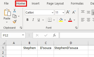
We can use the “&” operator in a formula to merge cells. For example, if we wish to merge cells B1 and C1, we can use the formula =B1&C1.
#2 Merging cells across multiple rows or columns
By default, Excel’s “Merge & Center” option will only merge cells within a single row or column. However, we can also merge cells across multiple rows or columns. For this purpose, select the cells we need to merge, right-click on the selection, and choose “Format Cells”. In the “Alignment” tab, check the “Merge cells” checkbox and select the number of rows or columns we want to merge. This will create a merged cell that spans multiple rows or columns.
#3 Using conditional formatting to highlight merged cells
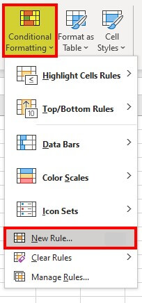
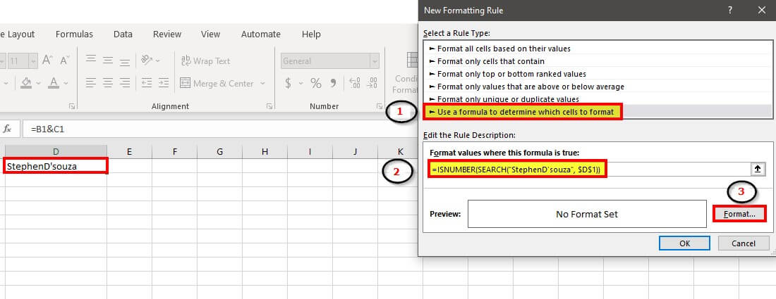
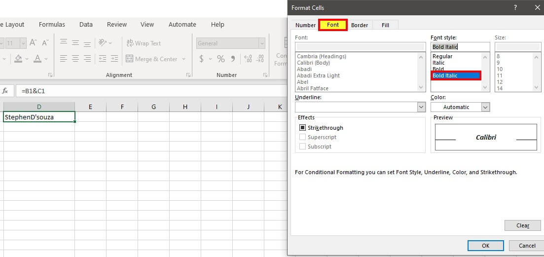
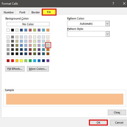
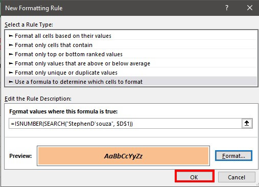
Merging cells can make applying conditional formatting to specific cells difficult since the merged cell acts as a single entity. However, we can use conditional formatting to highlight merged cells based on specific criteria. To do this, select the merged cell we need to format and choose “Conditional Formatting” from the “Home” tab. Select “New Rule” and choose the formatting criteria per the requirement. Choose “Use a formula to determine which cells to format“. After that, enter the formula referencing the merged cell.
For example, to highlight a merged cell that contains the word “StephenD’souza”, use the formula =ISNUMBER(SEARCH(“StephenD’souza”, $D$1)).
Alternatives to Merging Cells
Merging cells in Excel can sometimes cause formatting and sorting issues and make it difficult to enter data. Here are some alternatives to merging cells that you can try:
- Center-align text: We can center-align text across multiple cells without merging them. To do this, select the required cells you want to center-align, click on the “Alignment” group in the “Home” tab, and then click on the “Center Across Selection.”
- Wrap Text: We can also use the “Wrap Text” option to display text in multiple lines within a cell. This option is in the “Alignment” group in the “Home.”
- Column Width: We can increase the width of a column to fit the content without merging cells. To do this, drag the right border of the column header to the desired width.
- Conditional Formatting: We can use conditional formatting to highlight specific cells that meet certain criteria. This can happen without having to merge cells. For this purpose, select the cells we want to format, click on the “Conditional Formatting” option in the “Home” tab, and choose the formatting option that best suits our needs.
- Tables: Tables can help organize data to make it easier to view and work with without merging cells. We can create a table by selecting the data range and pressing “Ctrl + T” or by clicking on the “Table” option in the “Insert.”
How to Troubleshoot Common Issues with Merged Cells?
- Sorting: When merging cells, sorting data by column may not work as expected. To fix this, unmerge the cells and sort the data again. We can also try using the “Sort Left to Right” option in the “Sort & Filter” group on the “Data.”
- Alignment: Merging cells sometimes cause alignment issues, especially if the cells merged have different formatting. To fix this, select the merged cell and adjust the alignment settings, such as horizontal and vertical, to our liking.
- Data Entry: Merging cells can make it difficult to enter data, especially if the merged cell is not wide enough. To fix this, unmerge the cells and adjust the column width to fit the data. Alternatively, we can use the “Center Across Selection” option in the “Alignment” group on the “Home” tab to center-align the text across multiple cells without merging them.
- Formatting: Merging cells can sometimes cause formatting issues, such as merged cells having different fonts or colors. To fix this, unmerge the cells and apply the desired formatting to each cell.
Things to Remember
- Select the required cells to merge the cells horizontally and press “Alt + H + M + M” in sequence.
- Select the required cells to merge the cells vertically and press “Alt + H + M + V” in sequence.
- When we merge cells, the text in the upper-leftmost cell will remain the same, and the contents of the other cells will get deleted.
- If we merge cells that contain data, be sure to adjust the alignment and formatting of the merged cell to ensure that the data is correct.
- Lastly, note that the keyboard shortcuts for merging cells may vary depending on the version of Excel you are using.
Recommended Articles
This has been a guide to Shortcut Keys to Merge Cells in Excel. Here we discuss how to use Shortcut keys to Merge Cells in Excel, its limitations, practical examples, and downloadable Excel templates. You can also go through our other suggested articles –
