Introduction to Signal Processing in MATLAB
MATLAB is a programming environment that is interactive and is used in scientific computing. It is extensively used in a lot of technical fields where problem-solving, data analysis, algorithm development, and experimentation is required. The software which is discipline-specific is extensively written using MATLAB. In this article, we will study how signal processing is done in MATLAB. Mostly System objects are used in MATLAB to perform signal processing. We will see that in every processing loop, signals will be read and processed block to block or frame to frame. Also, the size of these frames can be controlled by us.
Before we see how signal processing is performed in MATLAB, let us quickly refresh our understanding of signal processing. Signal processing is used extensively to extract critical information present in detectors. We require the amplitude and timing of our output pulse to detect and measure the radiation. Signal processing techniques are required to extract all this information from low-amplitude and narrow-width pulses of the detector.
How Signal Processing is Performed in MATLAB?
Let us now learn how signal processing is performed in MATLAB.
Signal processing includes 3 main steps:
1. Initializing the streaming components
2. Creating the filter
3. Streaming and processing the signal
Let us understand all these steps one by one:
1. Initializing the streaming components
When initializing the streaming components, a variety of tools can be used to analyze signals in real-time. For portable applications, a handheld spectrum analyzer is often employed to monitor signal properties effectively. This tool complements MATLAB’s capabilities by providing a quick overview of frequency components before detailed processing in the software.
Code:
F = 3000;

[Setting the sample rate]
Object1 = dsp.SineWave('SamplesPerFrame',1024,...

'SampleRate',F,'Frequency', 200);

[Creating ‘sinewave’ object for generating the sine wave and setting the frequency to 200]
SA = dsp.SpectrumAnalyzer('SampleRate',F,'NumInputPorts',2,...

'ChannelNames',{'Input Wave'});

[Creating spectrum analyser to visualize the wave and setting the required properties]
Explanation: step 1 will create a sine wave of frequency 200Hz, as passed by us in the argument
2. Creating the filter
Here we will create a Notch peak filter
Code:
W = 1500;

[Setting the centre frequency of the filter]
Q = 35;

[Setting the Q factor to narrow the bandwidth of notch in filter]
B = W/Q;

[Setting the bandwidth]
NF = dsp.NotchPeakFilter('Bandwidth',B,...

'CenterFrequency',W, 'SampleRate',F);

fvtool(NF);

[Creating the Notch filter NF and setting the required properties]
Explanation: Step2 will result in creating a filter (notch peak), which we will use in the next step to filter our input signal.
3. Streaming and processing the signal
Code:
FV = [100 400 650 1100];

[Initializing frequencies for notch of the filter]
Index1 = 1;

[Setting the index of ‘for loop’]
VE = FV(Index1);

[The value of notch will be set to 100,400,650,and 1100 based on the change in value of VE in the for loop]
for Iteration = 1: 2000

[Creating the for loop which will repeat for 2000 iterations]
Examples to Implement Signal Processing Matlab
Below are some examples:
Example #1
Code:
Input = Object1();

if (mod(Iteration,350)==0)

if Index1< 4

Index1 = Index1+1;

else

Index1 = 1;

end

VE = FV(Index1);

end

NF.CenterFrequency = VE;

NF.Bandwidth = NF.CenterFrequency/     Q;

Output = NF(Input);

SA(Input,Output);

end

fvtool(NF)
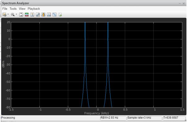
Output:
Example #2
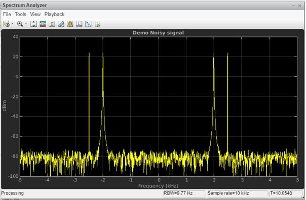
Let us take another example where we will create a noise signal from a sine wave.
Code:
Fre1 = 2000;

[Initializing the first frequency]
Fre2 = 2500;

[Initializing the second frequency]
F = 10000;

[Initializing the sample rate]
Object1 = dsp.SineWave('Frequency',[Fre1, Fre2],'SampleRate',F,...

'SamplesPerFrame',1026);

SA = dsp.SpectrumAnalyzer('SampleRate',F,...

'ShowLegend', false,'YLimits',[-100 40],...

'Title',‘Demo Noisy signal',...

'ChannelNames', {'Noisy Signal’});

[Creating spectrum analyser, to visualize the wave and setting the required properties]
for Iter = 1:200

input = sum(Object1(),2);

NI = input + (10^-4)*randn(1026,1);

[Creating the noisy signal]
SA (NI)

end
Output:
Example #3
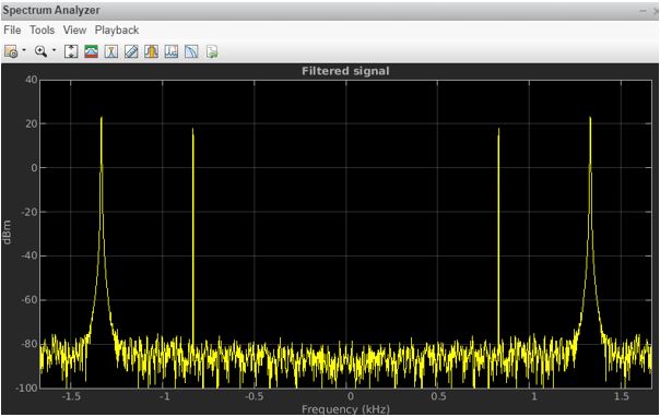
Now we can use a ‘multirate’ filter to tackle the noise created. For using a ‘multirate’ filter, we will first create a system object “DSP.FIRDecimator”.Next, we will need to create a new ‘System Analyser’ to view the filtered output. This is how our code will look like now:
Code:
x = designMultirateFIR(1,2,12);

[Initializing the multirate filter]
FD = dsp.FIRDecimator(3, x);

[Initializing the object FIRDecimator]
fvtool(FD);

Fre1 = 2000;

[Initializing the first frequency]
Fre2 = 2500;

[Initializing the second frequency]
F = 10000;

[Initializing the sample rate]
Object1 = dsp.SineWave('Frequency',[Fre1, Fre2],'SampleRate',F,...

'SamplesPerFrame',1026);

SA = dsp.SpectrumAnalyzer('SampleRate',F,...

'ShowLegend', false,'YLimits',[-100 40],...

'Title', ‘Demo Noisy signal',...

'ChannelNames', {'Noisy Signal’});

[Creating spectrum analyser to visualize the wave and setting the required properties]
SA2 = dsp.SpectrumAnalyzer('SampleRate', F / 2,...

'ShowLegend', false,'YLimits',[-100 40],...

'Title','Filteredsignal’,...

'ChannelNames', {'Filtered signal’});

[Creating another spectrum analyser to visualize the filtered wave and setting the required properties]
for Iter = 1:200

inp = sum(Object1(),2);

NI = inp + (10^-4)*randn(1026,1);

[Creating the noisy signal]
FO = FIRDecim(NI);

[Using the ‘multirate’ filter]
SA (NI)

SA2 (FO)

end
Output:
Conclusion
Signal processing includes analyzing the signal and taking the required actions. In this article, we learned how to analyze the signal and view it using Spectrum analyzer and how to filter a signal if required.
Recommended Articles
This is a guide to Signal Processing Matlab. Here we discuss an introduction to Signal Processing Matlab, how does it perform in steps with examples. You can also go through our other related articles to learn more –


