Updated May 29, 2023
Excel Slicer (Table of Contents)
What is Slicer in Excel?
Slicers in Excel is a tool that filters the data as per our need by slicing off a portion of data from the created table using the Pivot Table option in Excel. To apply Slicer, first, create a Pivot table as a table available under the Insert menu option. Then, in the same Insert menu tab, select Slicer, which is available under the Filters section. In the slicer connection box, we see an Insert Slicer box with all the available data headers used to create that Pivot Chart. Now, if we select any or multiple fields, we can get a slicer box on the screen. There, click on any data to filter the table.
How to Insert Slicer in Excel?
Let’s understand how to Insert Slicer in Excel with some examples.
Example #1 – How to Insert Slicer under Tables in Excel
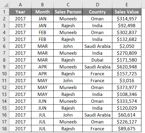
Suppose we have data on sales for the past two years, as shown below:
We will see how the slicers can be added to this data. Follow the steps given below:
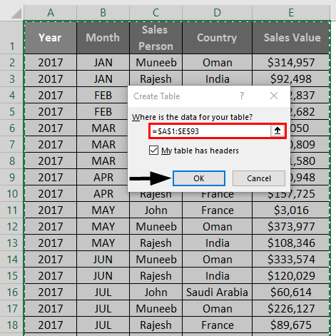
Step 1: Click on Insert tab > select Table under the Tables option menu.
- Select all the data across A1 to E93 and insert a table for these ranges. It will pop up a new window called Create Table with all the ranges we have selected to insert Table. Click on the OK button.
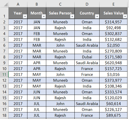
Your table should look like the one shown in the screenshot below.
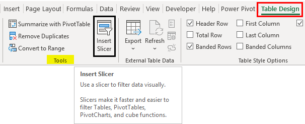
As soon as you insert a table, you’ll see a new tool added on the right-hand side of the upper ribbon pane under the Table Tools option named Table Design.
Step 2: Click on the Design tab to see a series of options under it. Click on the Insert Slicer button under the Tools section inside the Design tab. It will allow you to add slicers to the table.
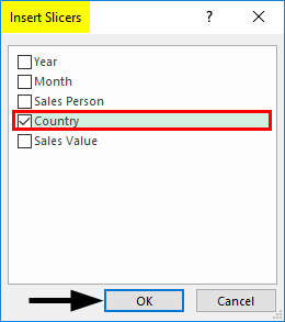
Step 3: Click the Insert Slicer button under the Tools option inside the Design tab, and you’ll see an Insert Slicer window. Inside it, you can have all the columns in the table and use any of them as a slicer. I will choose Country as a slicer option and see what happens. Click the OK button after selecting the Country as a slicer.
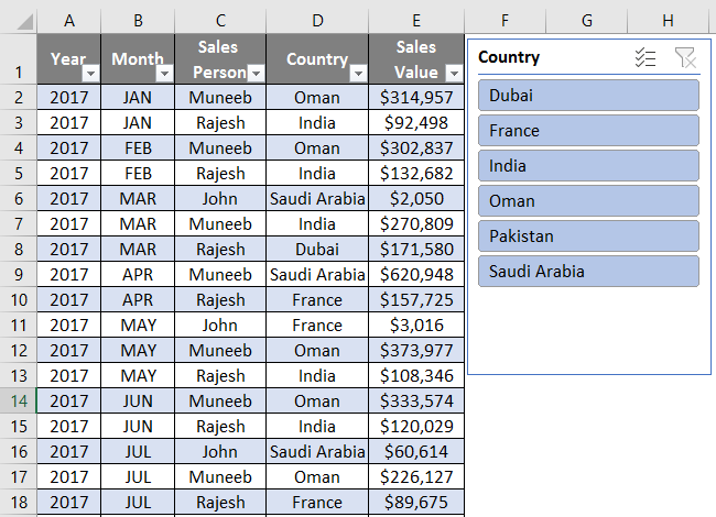
Step 4: You can see a slicer added under your Excel table with all country labels.
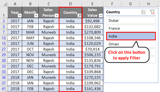
Step 5: You can use each country button to filter the data. For example, If I Want to see the data associated with India as a country, I just need to click on the India slicer button and see the magic. It will apply a filter on the table for all the rows with India as a country. See the screenshot below.
This is how we can apply the slicer to the Excel table.
Example #2 – How to Insert Slicers for Pivot Table Data
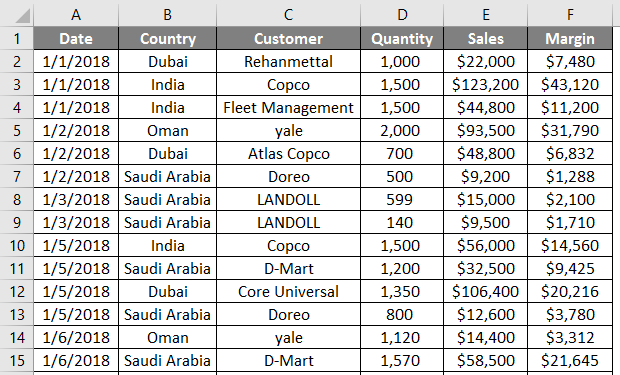
Suppose we have data on customer-wise sales for 2018 day by day, as shown in the screenshot below. This data accumulates 100 rows. See the partial screenshot below for your reference.
We would like to slice and dice this data first with the help of the Excel Pivot Table.
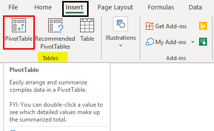
Step 1: Click on the Insert tab placed on the upper ribbon of the active Excel sheet. You will find out an option called PivotTable under the Tables section. Click on it to insert a pivot on the current working sheet.
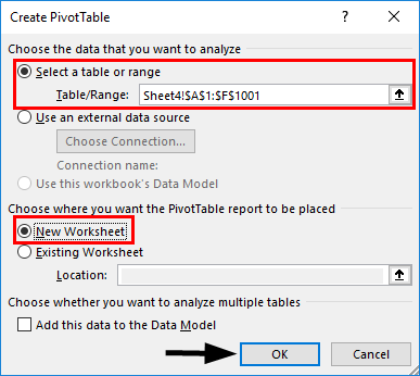
Step 2: A new window named Create PivotTable pops up as soon as you click on the PivotTable button under the Tables section. Select all the data as a Table/Range and select the location where the pivot will be added. Click OK once done. Please see the screenshot below.
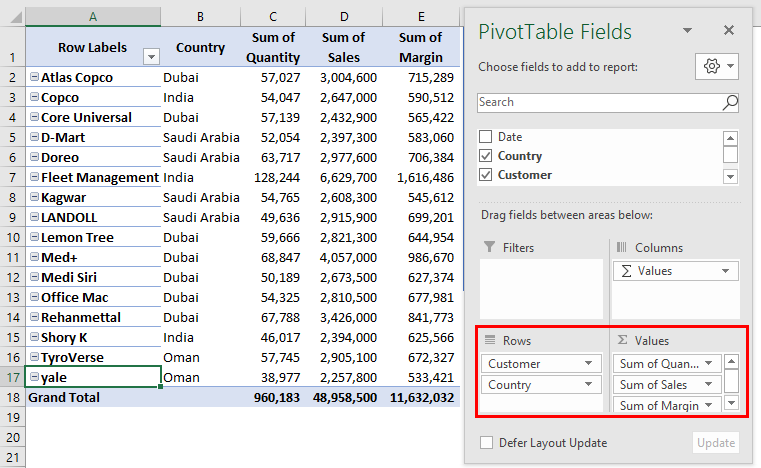
Step 3: Once you hit OK, the pivot table will successfully be added to the selected data ranges. Now you can choose the columns you want to see under the pivot layout. I will choose the following layout option.
- Rows: Customer, Country
- Values: Quantity, Sales, Margin
Please see the screenshot given below.
Now, we need to add the slicers for this pivot table. Let’s see how we can do that.
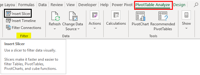
Step 4: As soon as you create a pivot table, you’ll see two new tabs active on the Excel ribbon: Analyze and Design. Click on Analyze tab out of those.
Step 5: There are different options available for analysis under this tab. Click the Insert Slicer button under the Filters section in Analyze tab to insert a slicer.
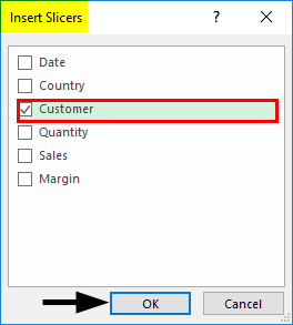
Step 6: As soon as we click on the Insert Slicers button, a new window pops up with all the column names present, based on which you can insert slicers on your pivot. Tick the one which you want to add as a slicer. I want to add the Customer column under Slicers and hit OK. See the screenshot below.
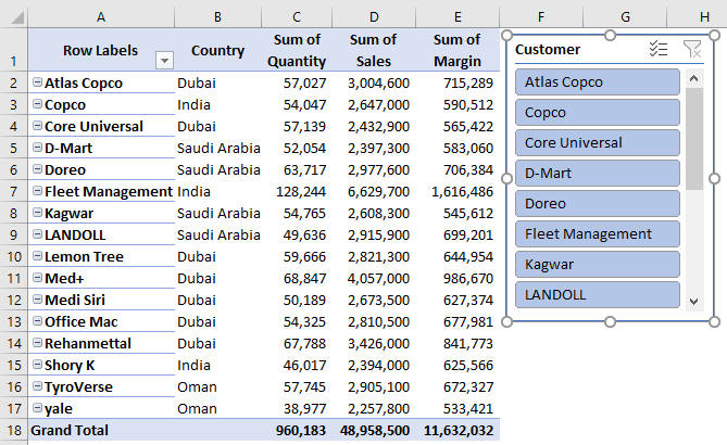
You can see a slicer of customers being added to your pivot. See the screenshot below.
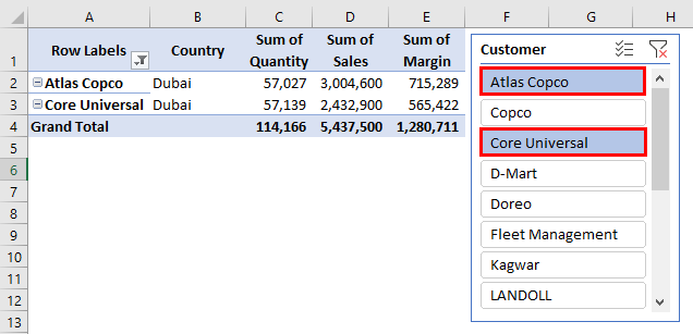
I can select the specific customer under the slicer or multiple customers simultaneously (hold the CTRL button and click on the customers one by one you want) and apply the filters on the pivot table.
This is how we can insert slicers under PivotTable. This is the end of this article. Let’s wrap things up with some points to be remembered.
Things to Remember About Slicer in Excel
- Slicers are dynamic filters that can be applied on Tables, Pivots, or PivotCharts.
- You can select more than one item under slicers. Hold the CTRL button and click one by one the slicers against which you want to slice data against.
Recommended Articles
This is a guide to Slicer in Excel. Here we discuss How to Insert Slicer in Excel, practical examples, and a downloadable Excel template. You can also go through our other suggested articles –
