Sort by color in Excel (Table of Contents)
Sort by color in Excel
In Excel, there are two ways to sort any data by Color. Firstly, we can sort the data by color through filters. For this, apply the filter selecting an option from the Data menu tab and then select the Sort by cell color or font color from the drop-down option. And other ways is sorting the data using the Sort option available in the Data menu tab. Once we select this, under Sort On the drop-down, we can select the sorting by cell color or by font color.
How to Use Sorting In Excel?
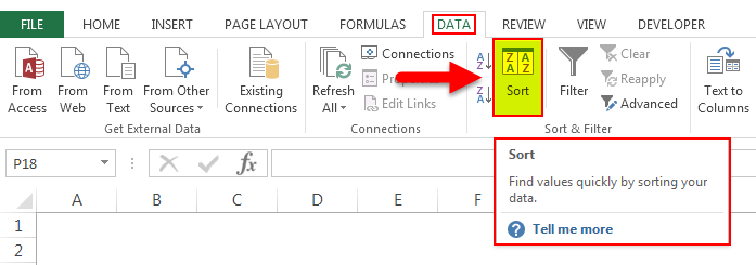
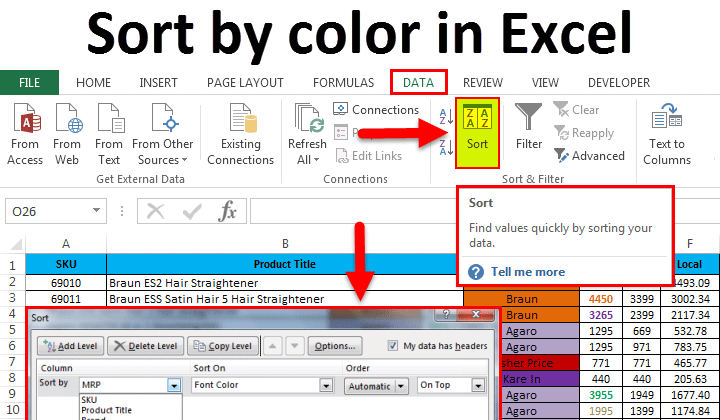
In excel, we can find SORT under the DATA menu, as shown in the below screenshot.
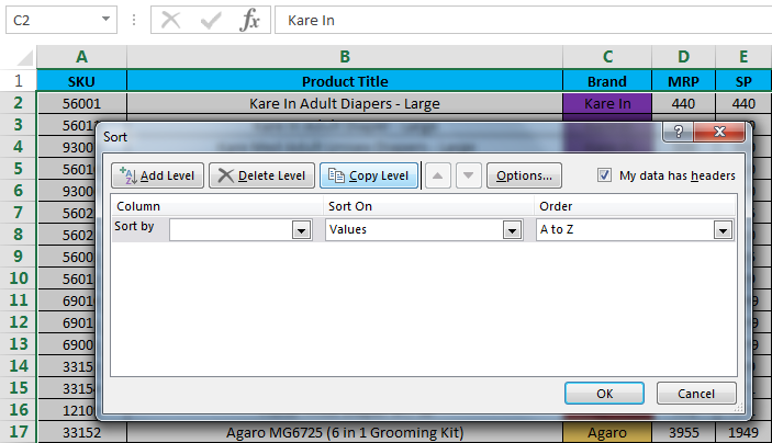
We can sort the data by color in excel in a simple way where we have a custom sort option in excel, here we can sort the data by multiple options like by Cell Color or by Value (Numbers) or by Font Color or by Cell Icon or by ascending or descending order. Once we click on the sort option, we will get the below dialogue box with multiple sorting as shown below.
Examples of Sort by color in Excel
In this example, we are going to see how to sort the data by color.
Example #1: Sort By Cell Color
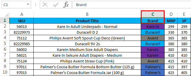
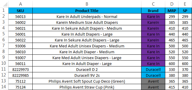
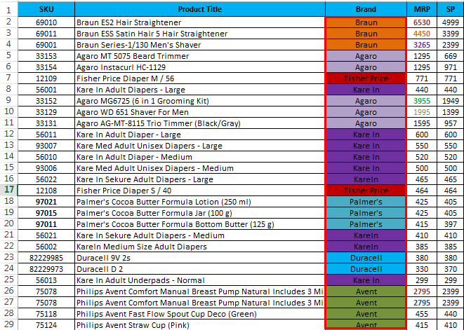
let’s consider the sales data, which has several categories like product name, Brand, MRP, Selling Price, Local, Zonal, National.
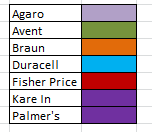
In sales data, we have categorized brands in specific colors so that they can be displayed easily, as shown in the below screenshot.
To apply sort by color in the sales data, follow the below steps.
- Select the C column named as Brand.
- Go to Data Menu and click Sort.
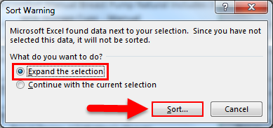
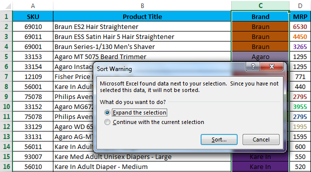
- Once we click the sort, the sorting feature will either expand the selection or ask the option, so select Expand the selection and click the Sort command button so that we will get multiple sorting options, as shown below.
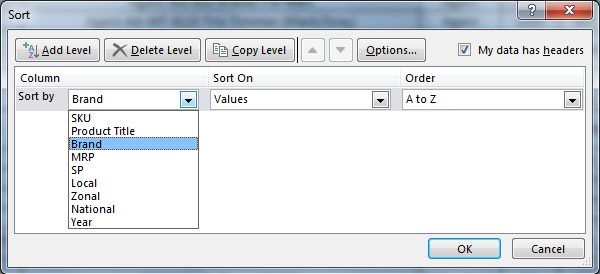
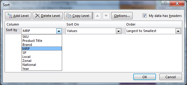
- We can see that sort by has various options that come from the sales data caption header like Brand, MRP, SP, Local, Zonal, National, Year.
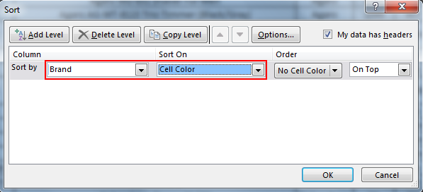
- Now let’s select sort by “Brand”, Select Sort on by Cell Color, so that we can sort the Brand by color.
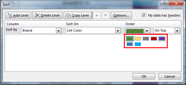
- Now select the order by color where the sorting option will show various colors that we have already mentioned for all brands. Hence we can select any color, so I have selected a purple color.
- Here the color purple represents the Brand name “Kare In”, so the brand will be sorted color-wise as shown below and select the option on top so that sorting will get the order by chosen color on top.
Example #2: Sort by Font Color
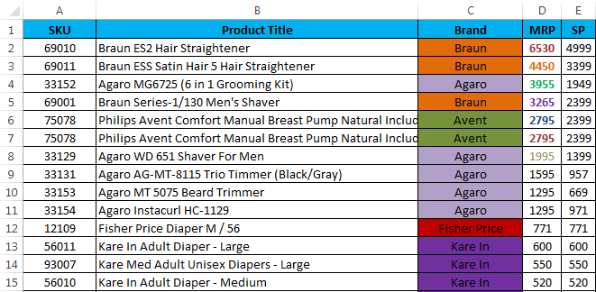
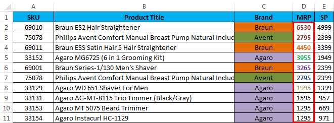
In this example, we will see how to do sorting by font color by using the same sales data where MRP has been highlighted as a specific colour that denotes highest to lowest MRP.
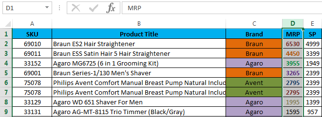
In the above sales data, we can see that MRP has been highlighted by font color, and we will do the sorting by font color as follows.
- Select the cell name MRP.
- Go to the Data menu and click Sort.
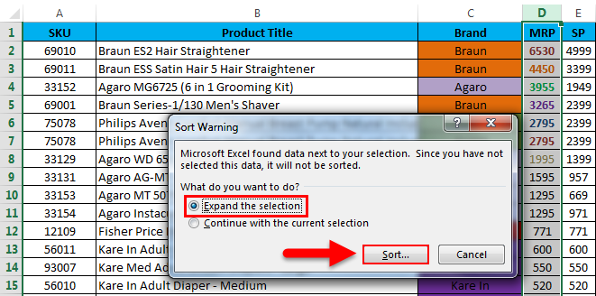
- Once we click Sort, the sorting feature will either expand the selection or ask the option as shown below. Choose ‘ Expand the selection ‘ and click the Sort command button.
- We will get the sorting dialogue box as shown.
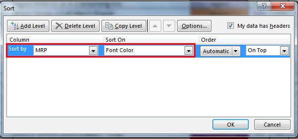
- Here select the Sort By option as MRP and Select the Sort On as Font Color.
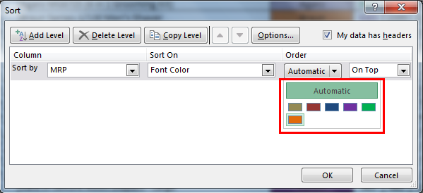
- Now select the order by Color, which shows several colors that we have mentioned for the highest MRP.
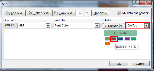
- Click on the font color for MRP, select the color Maroon, and choose the On Top option to get the chosen color so that sorting will be arranged by font color.
- Hence the MRP has been sorted by “Font color.”
Example #3
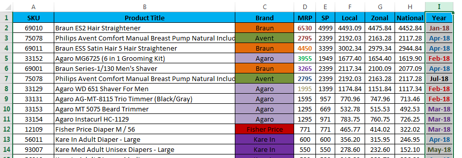
In this example, we will see how to sort font color Year wise where YEAR has been highlighted with several font colors, as shown in the below screenshot.
- Select the cell name I, which has the caption name as YEAR.
- Go to the Data menu and click Sort.
- Once we click Sort, the sorting feature will either expand the selection or ask the option. Choose expand the selection and click the sort command button.
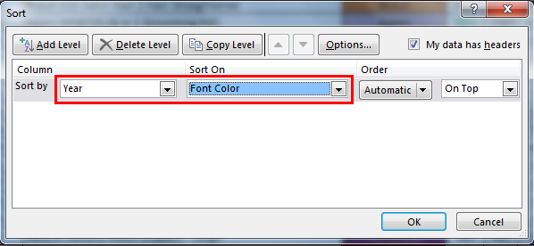
- We will get the sorting dialogue box as follows, now choose the Sort by option as Year and choose Sort On with Font Color.
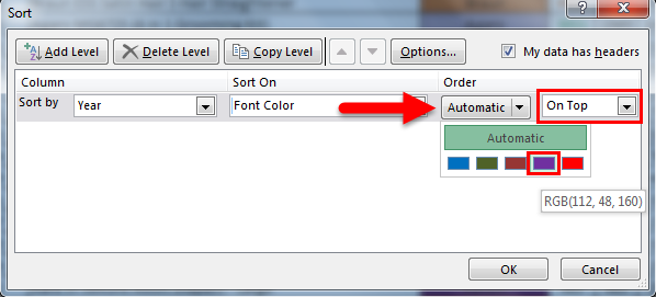
- We will get the option to choose font color as follows. Now choose the order by Font color, choose the On Top option to get the chosen color on top, and we will get the following result.
- The above sales data shows that “year” has been arranged with Font color as specified from Top.
Example #4
In the above examples, we have seen that sorting has been done with cell color and font color by selecting ON TOP.
Let’s consider the same sales data, and now we will see how the sales data appears if we select the order by On Bottom option as follows.
- Select the Brand column and apply the Sort option; sorting will ask to expand the selection or keep the current selection. So we will select the first option to Expand the selection.
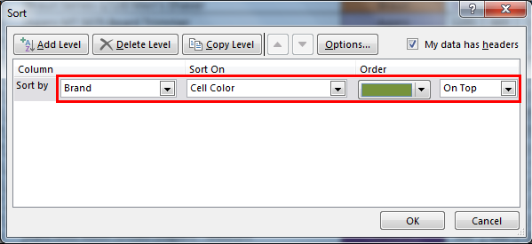
- Now we will get the below-sorting dialogue box as follows. As you can see, we have selected the sorting by “Brand” and Sort on “ Cell Color” and select as “Green Color”.
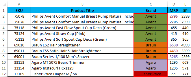
- Now we will get the results as shown below in the screenshot.
- We can see the sales data has been arranged Brand wise with the cell color “Green” by default. On Top selection has been chosen.
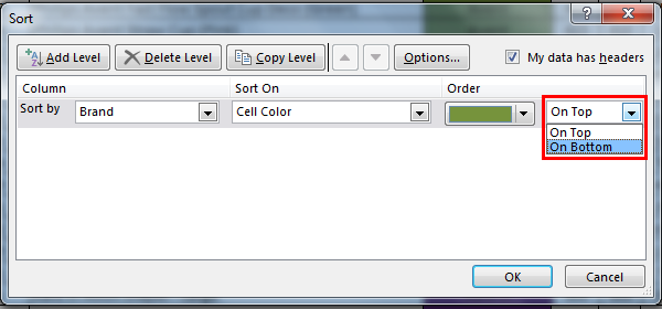
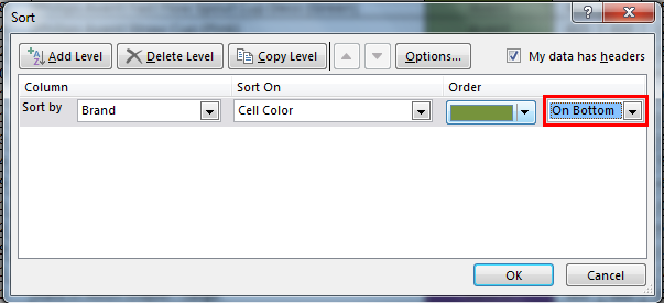
- Now select the On Bottom option to see how the sales data can be arranged from the bottom.
- We have chosen the On Bottom option so that the result will be shown from the bottom.
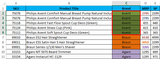
- In the below screenshot, we can see the difference that sales data has been arranged Brand wise with the cell color “Green” and the order by one BOTTOM.
Things to Remember
- While applying Sorting by color, make sure that all colors have been specified with different colors.
- Make sure that the “My data has the header” option has been check marked.
- Sort by color can be applied for only one color.
- We can sort the color with the On TOP or On Bottom option.
Recommended Articles
This has been a guide to Sort by color in Excel. Here we discuss the Sort by color in Excel and how to use the Sort by color in Excel, along with practical examples and a downloadable excel template. You can also go through our other suggested articles –
