State Space Model

Updated August 1, 2023

Introduction to State Space Model

State Space Model (SSM) is a powerful tool in various disciplines to simulate dynamic systems with hidden states. SSMs, initially developed in control engineering and then adapted for other applications, have proven indispensable in finance, economics, ecology, and signal processing. The purpose of this article is to provide a full review of the State Space Model, including fundamental ideas, applications, and estimating approaches.

Table of Content

• Introduction to State Space Model
• What is State Space Model?
• Key Components of State Space Model
• Applications of State Space Model
• Types of State Space Model
• Formulation of State Space Model
• Kalman Filter
• Model Validation and Selection
• State Space Model in Control System
• Example of State-Space Model by direct derivation
• Advantages of state-space Model

Key Takeaways

• The state-space analysis is a versatile and powerful framework for modeling and analyzing dynamic systems representing various system types.
• The framework supports improved control design, state estimates, and model validation, resulting in superior system performance and stability.
• The benefits of state-space analysis are its efficiency, real-time application, and capacity to provide insights into system behavior, controllability, and observability.

What is State Space Model?

State Space Model (SSM) is the behavior of dynamic systems over time using mathematical and statistical methods. They offer a flexible framework for modeling systems with hidden or unobservable states when only noisy or indirect observations of the system’s behavior are available. Control engineering, finance, economics, signal processing, ecology, and other disciplines extensively use state space model.

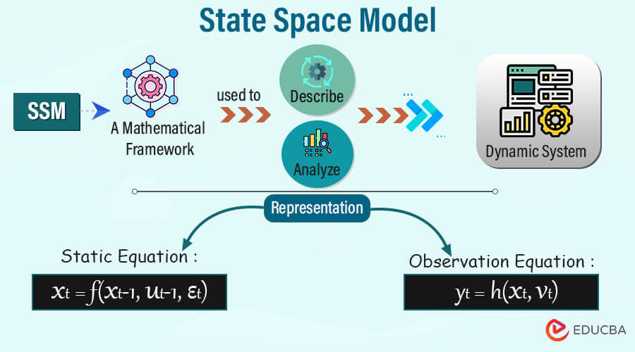
State Space Model consists of two fundamental equations: State Equation and Observation Equation.

Key Components of State Space Model

Below are some of the Key Components:

1. State Variables

State variables are a set of internal variables that characterize the current state of a dynamic system. They represent the system’s essential quantities, which are not directly observable but are crucial in determining its behavior over time. State variables are denoted by a vector, commonly represented as “x(t),” where “t” means the current time step. The number of state variables depends on the complexity of the system being modeled.

Example: In a simple linear mechanical system, the state variables could be the position and velocity of the system’s mass.

2. Observation (Measurement) Variables

Observation variables are the measurable quantities or outputs of the system. Unlike state variables, observation variables are directly observable or measurable. A vector denotes them, usually represented as “y(t),” where “t” denotes the current time step. The number of observation variables can vary depending on the available measurements from the system.

Example: In the linear mechanical system mentioned earlier, the observation variables could be the position measurements obtained from sensors.

3. Control Variables

Control variables are external inputs or control signals applied to the system to influence its behavior. An external agent can control these inputs to regulate or optimize the system’s performance. A vector denotes control variables, typically represented as “u(t),” where “t” denotes the current time step.

Example: The control variables in a temperature control system could be the heater power and fan speed.

4. System Dynamics Equations

The system dynamics equations describe the evolution of the state variables over time. They represent the underlying laws or principles that govern the system’s behavior. These equations are typically differential equations, either in continuous-time or discrete-time form, depending on the nature of the system and the modeling requirements.

Example (Continuous-time): The system dynamics equations for a simple mass-spring-damper system could be represented as follows:

Where “x” is the position, “v” is the velocity, “k” is the spring constant, “m” is the mass, “c” is the damping coefficient, and “u” is the control input.

5. Observation Equations

The observation equations relate the state variables to the observation variables. They define how the state variables are mapped to the measurable outputs of the system. Observation equations also account for any measurement noise or uncertainties in the measurements.

Example: For the simple mass-spring-damper system, the observation equation could be as follows:

where “y” is the measured position, “x” is the true position (state variable), and “n” is the measurement noise.

Applications of State Space Model

State Space Models (SSMs) have versatile applications across several fields and can manage complicated, dynamic systems with hidden states. Some well-known applications of State Space Models include:

• Control Engineering: Dynamic systems use SSMs to explain and predict their behavior, enabling the implementation of efficient control and feedback mechanisms. They are critical in applications like aerospace, robotics, and process control.
• Finance and Economics: State Space Model are essential in modeling financial time series, asset pricing, and economic factors. Risk management and portfolio optimization rely on their usage. Additionally, they aid in predicting stock prices, interest rates, and economic indicators.
• Time Series Analysis: State Space Models are an effective tool for analyzing time-dependent data such as temperature changes, traffic patterns, and economic trends. They help in the identification of underlying patterns, prediction, and estimation of missing values.
• Signal Processing: Regarding signal processing applications, SSMs are crucial in extracting reliable and helpful information from noisy signals and measurements. Speech recognition, picture processing, and communication systems all utilize them.
• Ecology and Environmental Studies: Researchers use State Space Models (SSMs) to investigate ecological systems, wildlife populations, and environmental factors. They help analyze species interaction dynamics, ecosystem modeling, and climate change.
• Health and Medicine: In epidemiology, pharmacokinetics, and disease modeling, researchers use state space models to predict disease transmission, optimize medicine doses, and analyze patient health trajectories.
• Robotics and Autonomous Systems: In robotics, researchers use SSMs for localization, mapping, and motion planning. They allow robots to determine their position and navigate unclear and changing environments.
• Speech and Natural Language Processing: Researchers use SSMs to improve the performance of language-based systems through speech recognition, language modeling, and machine translation.
• Economics and Finance: SSMs are used in economic analysis and decision-making by forecasting economic variables, modeling financial time series, and predicting asset prices.
• Neurosciences: SSMs help model brain activity and study brain dynamics in neuroimaging and brain signal analysis, resulting in new insights into cognitive processes and neurological illnesses.

Types of State Space Model

Based on the linearity of their state and observation equations, there are two types of State Space Models (SSMs):

1. Linear State Space Models (LSSMs)

Linear State Space Models (LSSMs) are a sort of State Space Model in which the state and observation equations are expressed as linear functions of the state variables and observations.

The general form of a Linear State Space Model can be expressed as follows:

State Equation (State Transition Model):

Where,

• x_t: At time t, the state vector represents the system’s hidden or unobservable variables.
• A_t: A state transition matrix is a matrix that connects the state at time t to the state at time t-1. It captures the dynamics of the system.
• x_{t-1}: State vector at time t-1.
• B_t: At time t, the control input matrix accounts for any external control or effect on the system.
• u_t: Control input vector at time t.
• w_t: Process noise represents the uncertainty or random fluctuations in the state transition process.

Observation Equation:

Where,

• y_t: At time t, the observation vector represents the system’s measured or observed variables.
• C_t: The observation matrix maps the state vector to the observation space. It expresses how the states are related to the observable quantities.
• v_t: Observation noise, which accounts for measurement errors and uncertainty in the observed data.

Key characteristics:

• Linearity: The state and observation equations are linear functions, resulting in closed-form solutions and efficient computing.
• Gaussian Assumption: LSSMs often assume Gaussian processes and observation noise, simplifying estimation and enabling the application of Kalman filters and smoothers.
• Recursive Estimation: Recursive algorithms such as the Kalman filter are supported by LSSMs, allowing for real-time state estimation and prediction as new observations become available.
• Optimal Filtering: The Kalman filter and smoother are optimum linear estimation techniques that provide the best linear unbiased estimate of the state in the presence of noisy observations.

2. Nonlinear State Space Models (NSSMs)

Nonlinear State Space Models (NSSMs) express the state equation, observation equation, or both as nonlinear functions of state variables and observations. Unlike Linear State Space Models (LSSMs), NSSMs do not have closed-form solutions and frequently require more complex numerical approaches for estimate and inference.

The general form of a Nonlinear State Space Model can be expressed as follows:

Nonlinear State Equation (State Transition Model):

Where,

• x_t: At time t, the state vector represents the system’s hidden or unobservable variables.
• f: The nonlinear state transition function describes how the state at time t is affected by the state at time t-1 and any control inputs u_t.
• x_{t-1}: State vector at time t-1.
• u_t: Control input vector at time t.
• w_t: Process noise represents the uncertainty or random fluctuations in the state transition process.

Nonlinear Observation Equation:

Where,

• y_t: At time t, the observation vector represents the system’s measured or observed variables.
• h: A nonlinear observation function maps the state vector to the observation space. It describes how the states are related to the observable quantities.
• v_t: Observation noise, which considers measurement mistakes and uncertainty in observed data.

Key characteristics:

• Nonlinearity: At least one of the state or observation equations has nonlinear functions, making the model more expressive and capable of handling complicated system interactions.
• Numerical Estimation: Using numerical methods such as the Extended Kalman Filter (EKF), Unscented Kalman Filter (UKF), or Particle Filter (PF) is often necessary to estimate the states and parameters of NSSMs.
• Particle Filtering: In NSSMs, we often use particle filters to estimate the posterior distribution of states. This allows for more precise inference in highly nonlinear and non-Gaussian environments.
• Flexibility: NSSMs can model more real-world systems than LSSMs since linearity assumptions do not restrict them.

Formulation of State Space Model

A State Space Model (SSM) is created by defining the model’s core components and expressing them mathematically. A State Space Model usually consists of state equations and observation equations.

1. State Equations

The state equations represent the evolution of the system’s hidden or latent states over time. These states are not readily visible, yet critical to understanding the system’s behavior. The state equations are typically given in recursive form, allowing the model to anticipate the states at each time step based on the previous states and any control inputs.

The general form of state equations is as follows:

Where,

• x_t​ represents the state vector at time t.
• f is the state transition function, which specifies how the states evolve. It is often a nonlinear function.
• x_t−1​ is the state vector at the previous time step (t−1).
• u_t−1​ indicates any control inputs or external influences impacting the state transition at time t−1.
• ϵ_t​ is the process noise and captures the uncertainty and stochasticity of the state transition process.

2. Observation Equations

The observation equations represent the link between the latent states and the observed measurements. These are typically linear or nonlinear functions that connect the hidden states to the observable outputs at each time step.

The general form of observation equations is as follows:

Where,

• y_t represents the observed output (measurement) vector at time t.
• ℎ is the observation function that connects the states to the observed measurements. It can be both linear and nonlinear.
• x_t​ is the state vector at time t.
• v_t is the observation noise, which accounts for measurement errors and uncertainties.

Kalman Filter

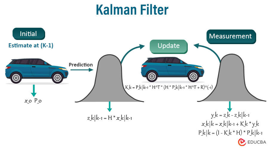
The Kalman filter is a recursive algorithm for estimating linear dynamic systems’ states. The system can derive an optimal estimation of its state by combining measurements and predictions while accounting for measurement noise and process noise. Here’s an explanation of the Kalman filter with an example:

Example: Tracking the Position of a Moving Car

Consider a basic scenario in which we want to track the position of a car moving in one dimension (for example, along a straight road). Our sensor delivers noisy car position measurements at discrete time intervals. A constant velocity model can describe the motion of the car:

• State Variables: Position (x): The car’s position along the road. Velocity (v): The speed of the car.
• State Transition Equation (System Dynamics): The state evolves with a consistent velocity over time. State update equation: x(k+1) = x(k) + v(k) * Δt Here, Δt is the time elapsed between two consecutive measurements.
• Observation Equation (Measurement Model): The measurements are noisy and indicate the car’s location. Measurement equation: z(k) = x(k) + w(k) Here, z(k) is the noisy measurement at time step k, and w(k) is the measurement noise.

Now, let’s use the Kalman filter to estimate the car’s position and velocity at each time step.

Steps of the Kalman Filter:

• Initialization: Initialize the state vector and covariance matrix with initial estimations. Assuming we know the car’s initial position (x0) and velocity (v0), the initial covariance matrix P0 is set based on uncertainty.
• Prediction Step: Project the current state beforehand using the state transition equation. To account for uncertainty in the prediction step, compute the process noise covariance matrix Q. Predicted state: x̂(k+1|k) = x(k) + v(k) * Δt Predicted covariance: P(k+1|k) = P(k) + Q
• Update Step: Incorporate the new measurement into the state estimate to update it and reduce uncertainty. Compute the measurement noise covariance matrix R based on the sensor noise characteristics. To identify the balance between prediction and measurement, calculate the Kalman gain K. Update the state estimate: x̂(k+1) = x̂(k+1|k) + K(k+1) * [z(k+1) – x̂(k+1|k)] Update the covariance matrix: P(k+1) = (I – K(k+1)) * P(k+1|k)
• Repeat: Return to the prediction step and proceed with the next measurement.

Example Output:

Suppose we begin with an initial location of x0 = 0 and a velocity of v0 = 10 m/s. At each time step, we obtain the following noise measurements:

• z1 = 3 (measurement at time step 1)
• z2 = 8 (measurement at time step 2)
• z3 = 12 (measurement at time step 3)

The Kalman filter will offer state estimates (position and velocity) at each time step. The system will update its predictions as soon as new measurements are obtained, provided that the process noise covariance matrix Q and the measurement noise covariance matrix R have appropriate values.

Model Validation and Selection

Model validation

To validate a model, its accuracy is assessed using data not used during its training phase. The purpose is to evaluate the model’s generalization capacity and ability to produce accurate predictions on new, unseen data. It helps identify potential problems impacting model performance, such as overfitting or underfitting.

Standard techniques for model validation include:

• Train-Test Split: We divide the dataset into two parts: a training set to train the model and a separate test set to evaluate its performance.
• Cross-Validation: We divide the dataset into various subsets (folds) and train and test the model multiple times, rotating the subsets for training and testing.
• Leave-One-Out Cross-Validation (LOOCV): In this type of cross-validation, we consider each data point as a separate test set and train the model on all other data points.
• K-Fold Cross-Validation: Dividing the dataset into K subsets, we train and test the model K times, with each iteration utilizing a different subset for testing.

Model Selection

Model selection is comparing various candidate models to find the one that best matches the data and exhibits the best generalization performance. When working with several models or model architectures, choosing one that strikes the right balance of complexity and accuracy is crucial.

Key considerations for model selection include:

• Complexity: A model should have enough complexity to capture the underlying patterns in the data but be simple enough to overfit or become computationally expensive.
• Performance Metrics: Use appropriate evaluation metrics to compare model performance, such as accuracy, precision, recall, F1-score, mean squared error (MSE), or other domain-specific metrics.
• Occam’s Razor: When simpler models perform equally well as more complicated models, choose them. According to Occam’s Razor, the simplest explanation (model) that fits the evidence is frequently the best.
• Bias-Variance Tradeoff: Consider the tradeoff between bias and variance: high-bias models may underfit the data, while high-variance models may overfit.
• Cross-Validation: Model validation techniques, such as cross-validation, allow us to evaluate the generalization performance of each candidate model.
• Domain Knowledge: Consider domain-specific insights and considerations that may guide model selection.

State Space Model in Control System

State space models are essential in control systems because they provide a robust framework for describing and analyzing dynamic systems. A state space representation in control theory allows us to model the evolution of a system’s internal state and its relationship with inputs and outputs.

Let’s examine an example of using the state space model in control systems:

Inverted Pendulum Control

Consider an inverted pendulum system with a pendulum attached to a movable cart. The purpose is to control the cart’s location so the pendulum remains balanced in an inverted position. The system’s control input is the force applied to the cart, and the output is the pendulum’s angle.

1. State Variables

To model a system as a state space model, we must define the state variables that describe the system’s internal state. We can select the following state variables for the inverted pendulum system:

• x1: Position of the cart (horizontal position)
• x2: Velocity of the cart
• x3: Angle of the pendulum (measured from the vertical position)
• x4: Angular velocity of the pendulum

2. State Transition Equation (System Dynamics)

The cart and pendulum motion equations define the system’s dynamics. These equations can be expressed in state space form as follows:

Where:

• F: Control input (force applied to the cart)
• m: Mass of the pendulum
• M: Mass of the cart
• l: Length of the pendulum
• g: Acceleration due to gravity

3. Observation Equation (Measurement Model)

The system’s measurements are often noisy but provide information regarding the pendulum’s angle. You can write the observation equation as:

4. Control Objective

To keep the pendulum balanced upright, the control objective is to create a control law that applies the proper force (F) to the cart depending on the measured pendulum angle (y).

5. Control Design

The state space model can be used to construct a control law using a variety of control approaches, such as state feedback control, LQR (Linear Quadratic Regulator), or pole placement. The control law seeks to achieve system stabilization and the desired behavior.

For instance, the following could be the creation of the control law in state feedback control:

Where x is the state vector, and K is the control gain matrix. The control gain matrix K is established based on the required closed-loop poles, which specify the system’s stability and performance characteristics.

Control systems can keep a balanced inverted pendulum by utilizing feedback from the pendulum angle and applying control law. State space model are a concise way to represent system dynamics, making designing effective control strategies for real-world applications possible. The principles behind state space modeling can help solve various control problems in different domains.

Example of State-Space Model by direct derivation (Mechanical Translating)

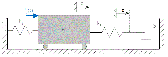
Consider the example below and derive a state-space model for the figure below. The input here is fa, and the output is y.

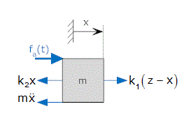
we can derive free body equations at two points from the above-shown figure, x and y.

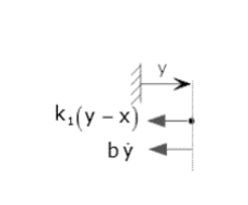
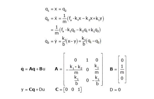
We have three energy storage elements in the above figure, so we obtain three state equations. Here, the energy-storing elements are the spring k2, the spring k1, and the mass m. So our state variables will be x and y.

q1 = x
q2 = x
q3 = x

Now, we need to find equations for these derivatives. The motion equations from the free body diagram when input u = fa are,

Advantages of State Space Model

Below are the different advantages:

• Flexibility: A wide variety of complex systems, including linear, nonlinear, time-varying, and multivariable systems, can be modeled using state-space techniques.
• Comprehensive Description: They offer a thorough and concise description of how a system’s internal state changes over time and how it interacts with inputs and outputs.
• Control Design: State-space model makes building sophisticated control strategies like state feedback and optimum control easier, improving the system’s performance and stability.
• State Estimation: Kalman filters and other methods can accurately and effectively estimate the state of a system by utilizing the state-space framework.
• Model Validation: State-space model enables thorough model selection and validation using various validation techniques, ensuring reliable model performance on unseen data.
• Real-Time Applications: State-space models can be used for real-time control and estimation in engineering and robotics since they are computationally efficient.
• System Analysis: State-space analysis provides insights into system behavior, stability, controllability, and observability, assisting in system diagnosis and optimization.
• Multidisciplinary Applications: They have applications ranging from engineering and economics to biology and finance, making them versatile modeling and control tools.

FAQs

Q1. What is Maximum Likelihood Estimation (MLE)?

Ans: MLE is a statistical method for estimating the parameters of a model by maximizing the likelihood function, which assesses the likelihood of observing the data given in the model. MLE delivers accurate and consistent parameter estimates.

Q2. What is the difference between the Kalman filter and the Extended Kalman Filter (EKF)?

Ans: We utilize the Kalman filter to estimate the state of linear dynamic systems. However, the Extended Kalman Filter (EKF) is an extension capable of handling certain types of nonlinear systems. The EKF accomplishes this by linearizing nonlinear functions for state prediction and update steps, making it a suitable solution for nonlinear state space models. 

Q3. How are state space models different from transfer function models?

Ans: State-space and transfer function models are popular dynamic system representations. The key distinction is that state space models describe the system in terms of internal state variables and their evolution through time. In contrast, transfer function models directly connect the input-output relationship without considering internal states.

Conclusion

State-space models provide a versatile and elegant framework for modeling and analyzing dynamic systems in various domains. They allow precise modeling, effective control design, and accurate state estimates. Due to their wide applications, state-space models are crucial for comprehending and modifying complex systems.

Recommended Articles

We hope this EDUCBA information on the “State Space Model” benefited you. You can view EDUCBA’s recommended articles for more information.

1. System Models
2. People Capability Maturity Model
3. Analysis Modeling
4. Data Modeling in MongoDB