Updated March 23, 2023
Introduction to Statistical Analysis Method
Statistical Analysis is the science of collecting, exploring, organizing and exploring patterns and trends using its various types, each of the types of these statistical analysis uses statistic methods such as, Regression, Mean, Standard Deviation, Sample size determination and Hypothesis Testing. It is results in the output that is used by the organizations to reduce the risk and predict the upcoming trends to make their positions in the competitive market.
Basic Fundamental Methods
Few of the basic fundamental’s methods used in Statistical Analysis are:
1. Regression
It is used for estimating the relationship between the dependent and independent variables. It is useful in determining the strength of the relationship among these variables and to model the future relationship between them. It has multiple variants like Linear Regression, Multi Linear Regression, and Non-Linear Regression, where Linear and Multi Linear are the most common ones. It offers numerous applications in discipline, including finance.
For Example
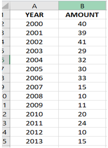
Suppose you are asked to predict how much snowfall will happen this year. Knowing the fact that global warming is reducing the average snowfall in your city. You are provided with the following tabular data of the year with respect to the amount of snowfall that happened each year in inches. Looking at the table you can estimate that the average snowfall will be 20-40 inches, which is a fair estimate but this can be even better-using regression.
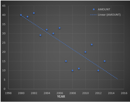
Since regression is fitting points to the graph, look at the following graph, From the regression line, it is clear to visualize that our initial estimate of 20-40 inch for 2015 is nowhere closer to the possible value. Since following the regression line, we can estimate that the snow falls for the year 2015 will be somewhere around 5-10 inches. Along with this, estimation regression also provides the line equation which in this case is:
y = -2.2923x + 4624.4.
This means that we can plug in the year as x value in the equation and get the estimate for that year.
Let’s say:
if you want to predict the snowfall in the year 2016 then by putting 2016 in-place of x we get:
y = -2.2923*2016 + 4624.4
= 3.132 inches.
2. Standard Deviation
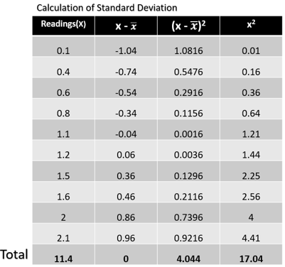
Standard deviations measure how the data are concentrated around their mean. More concentration will result in a smaller standard deviation and vice-versa. In other words, we can say that it is the summary measure of the difference of each observation from the mean. If we add the differences, the positive would be exactly equal to the negative and adding both will result is zero. In order to calculate the standard deviation, we need the computer the variance first. Variance is a measure of how far the set numbers are spread out. Let’s understand this by computing the variance and standard deviation of the table below:
In the given table we have 10 readings. To get the variance, the sum of the square of the differences (or deviations from the mean) i.e. 4.044 is divided by the total number of observations minus one. Thus,
Substituting the value from the table we get,
Variance = 4.044/10 = 0.4044
Finally, to get the standard deviation we take the square root of the deviation i.e.
Which is equal to 0.4044 = 0.6359
3. MEAN
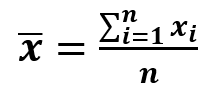
Mean is the sum of the list of numbers divided by the total number of items on the list. It is also known as the average. Assume that we have 3 different ratings for a movie. First is 7.0, The second rating is 9.0, and the third 6.0. The mean of these ratings is calculated by summing up these ratings and then dividing it by the number of ratings.
It is given by the formula:
Where: n: Number of elements
x: element
x̄: mean
So, the mean of the movie rating will be (7.0+9.0+6.0)/3 = 7.33. Now this mean value is used as the basis for comparison with other ratings. A rating that is above 7.33 is said to be rating is above average and for a rating below 7.33 is said to be the rating of below average. This mean is further used in the calculation of the standard deviation as you have seen above.
4. Sample Size Determination
Sample size determination as the name suggests is the samples of the dataset which is used for the analysis of data. This technique is useful when we have a large amount of dataset and we don’t want to go through each feature of the dataset. Instead of that, we select few data from the dataset such that those data are not bias. The whole idea is to get the right amount of data for the samples, because if that is not current then the whole data analysis will be affected. So, determining sample size is an important issue because a large sample size will result in a waste of time, money, and resource while a small sample size will result in an inaccurate result. In many cases, it is easy to determine the minimum size of the sample to estimate a process parameter.
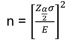
When sample data is collected, and a sample is computed then mostly the sample mean is different from the population mean. The difference between sample and population mean can be termed as an error. The margin of this error is given by:
where: population standard deviation
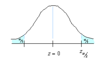
n: sample size: critical value. The region marked by its shows in the figure.
Rearranging the above formula, we can get the value of n i.e. the number of required sample sizes.
For Example, Our problem is that we need to estimate the average household usage of the Internet in one week. So, how much households must be randomly selected such that to make sure that 95% of the sample mean of time is within 1 min of the population mean? Assuming that from the previous survey we got = 6.95 minutes.
Solution:
We need to find n.95% confidence means = 0.05. Each of the shaded tail has an area of = 0.025. So, the region to either side of is 0.5-0.025 = 0.475. In a normal distribution, an area of 0.475 corresponds to 1.96 and therefore the critical value is = 1.96.
Margin Error E is 1 and = 6.95. Substituting these values in the equation of sample size we get:
Hence 186 households need to be randomly selected so as to make sure that 95% of the sample mean of time is within 1 min of the population means.
5. Hypothesis Testing
In this testing, we determine whether a premise is true for the dataset or not. Analyst test the samples with the goal of accepting or rejecting the null hypothesis. Statistical Analyst starts the examinations with a random number of populations. The null hypothesis is the value that the analyst believes to be true and the alternate to be false.
For example, if a person wants to prove that a coin has a 50% chance of landing on heads, then the null hypothesis will be yes, and the alternate hypothesis will be no. Mathematically, we can represent the null hypothesis as Ho: P=0.5. And the alternate hypothesis can be denoted by Ha.
100 coins flips are taken from the random population of coins and then the null hypothesis is tested. Now if we see that the 100 coins flip is taken as 40 head and 60 tails then the analyst can conclude that the coin does not have a 50% chance of landing on the head and will accept the alternate hypothesis and reject the null hypothesis. After which a new hypothesis would be tested, and this time the penny has a 40% chance of landing on the head.
Conclusion – Statistical Analysis Methods
In this article, we learned about a few fundamental statistical analysis methods, along with which we saw an example of how to use it. These methods are enough for you to kick start in the field of statistical analysis methods. Try to use these techniques on the different datasets to get more insight into them and to explore the analyst in you.
Recommended Articles
This is a guide to Statistical Analysis Methods. Here we discuss the fundamental statistical analysis methods along with the examples. You may also look at the following article to learn more –
