Updated June 7, 2023

Introduction to Step Function Matlab
The step function in Matlab is used for design control. We used to step and unit steps for immediate plotting of scalar input without using any particular toolbox in Matlab. A discontinuous function has zero value for a negative argument and has one value for a positive argument called a unit step function. We can apply the step function along with any other function, also called a system function. Once the system function is defined, then we can pass this function through the step function.
Syntax:
The syntax for Step Function Matlab is as shown below:
Step (sys)How to do Step Function Matlab?
Here we will see how to write a Matlab code for generating an advanced or delayed unit step function.
The steps are as follows:
Step 1: Take interval from user or decide by programmer.
Step 2: Take user or programmer choice either advanced or delayed function.
Step 3: Define time axis.
Step 4: Create a zeroth row vector to avoid garbage value.
Step 5: Write the unit step command.
Step 6: Finally, plot the function.
We also plot a transfer function response by using a step function.
The steps are as follows:
Step 1: Take a numerator in a variable.
Step 2: Take the denominator in another variable.
Step 3: Generate the transfer function using the ‘tf’ function and assign it to the sys1 variable.
Step 4: Use the step function to plot a response.
Examples of Step Function Matlab
Given below are the examples :
Example #1
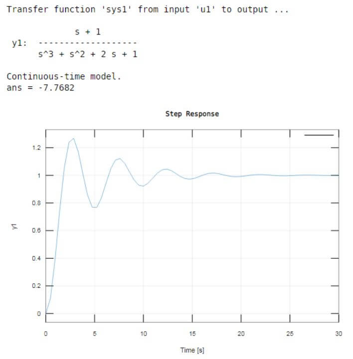
In this example, we learn how to use the step response functionality in matlab to plot the step response of the transfer function; we have G1 of s equals to s plus 1 divide by s cube plus s square plus 2s plus 1. Now we need to input this step function in a format that matlab understands, and we do that by writing down the vectors that represent the numerator and numerator. So we take two variables to represent the numerator and denominator, and these variables are num1 and den1, respectively. So, the numerator here is a num1 = [ 1 1 ], first 1 corresponds to s, and 2nd 1 corresponds to constant. The denominator here is den1 = [ 1 1 2 1 ], 1st one corresponds to s cube, 2nd one corresponds to s square, 2 corresponds to s, and the last 1 corresponds to the constant. Then we take sys1 equals to TF is a standard function for generating a transfer function in the s domain; s domain is a laplace domain given numerator (num1) and denominator (den1). There we have a transfer function in the sys1 variable. Now we use a step function to plot the step response of a system. Then we also use a grid function to look at grids on a plot.
Code:
clc;
close all;
clear all;
num1 = [ 1 1 ];den1 = [ 1 1 2 1 ];sys1 = tf (num1, den1)step(sys1)grid on
Output:
Example #2
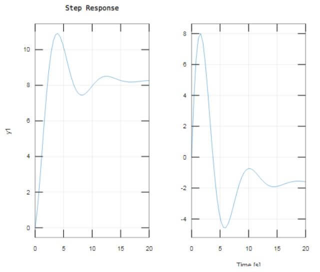
Let us see an example; we plot a 2nd order state–space model in this example. We take 4 variables, a1, b1, c1, and d1 which are Nx-by-Nx real- or complex-valued matrix. In our example, the value of d1 is zero. And these 4 variables are passed from the ss function; ss is a state space model. sys1 = ss (a1,b1,c1,d1) creates the discrete-time state-space model object of the following form: x[n+1]=a1x[n]+b1u[n] and y[n]=c1x[n]+d1u[n]. And this assigns to sys1. And then, we plot the response using a step function; it shows two responses.
Code:
clc;
close all;
clear all;
a1 = [-0.55, -0.78; 0.78,0];b1 = [1,-1;0,2];c1 = [1.96, 6.44];d1 = 0;sys1 = ss(a1, b1, c1, d1);step(sys1)grid on
Output:
The left plot shows the step response of the first input channel, while the right plot displays the step response of the second input channel.
Example #3
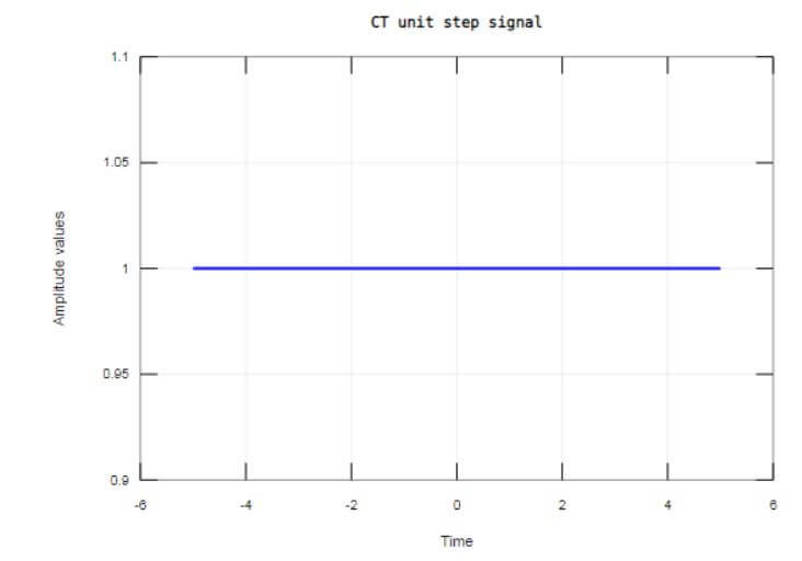
Let us see an example for generating a delayed or advanced unit step signal; 1st, we ask a user to enter an interval for which you want to get a step signal; for taking user values, we use an input function, which requests the user input and that number into which user entered that stored in an equitant variable. We also ask the user to close that the signal is delayed (+ve no.) or advanced (-ve no.). Then, in the x1 variable, we define a time axis. Then, to avoid trash values, we generate the zeroth row vector, which equals the unit step_CT variable. Then, we utilize a plot function to draw a unit step based on whether it is delayed or advanced. Then, using the xlabel and ylabel functions, we label the figure as the x-axis is time and the y-axis is amplitude. And using the title function, we give a title to that response. And we also use a grid function to display the grid on the plot.
Code:
clc;
close all;
clear all;
n = input('Enter the interval for which you want to get unit step signal: - ');
d = input ('Enter the delayed (+ve no. ) or advanced ( -ve no. ):- ');
x1 = -5:0.01:5;
unitstep_CT = zeros(size(x1));
unitstep_CT(x1>=0 + (d)) = 1;
plot(x1,unitstep_CT,'b','linewidth',2);
xlabel('Time');
ylabel('Amplitude values');
title('CT unit step signal');
grid on
Output:
Conclusion
In this article, we saw the concept of the Step function in Matlab. People use the step function for control design. I then observed the syntax related to the step function and learned how to use it in Matlab code. Also, we saw some examples related to the Step function and its output on matlab.
Recommended Articles
We hope that this EDUCBA information on “Step Function Matlab” was beneficial to you. You can view EDUCBA’s recommended articles for more information.


