SUBTOTAL Formula in Excel
In this article, we will learn about SUBTOTAL Formula in Excel. The function that returns a subtotal from a list or database can be defined as the Subtotal function.
Subtotal is a special function among other Excel functions because it can perform multiple operations, unlike other Excel functions that typically execute a single specific operation. Still, the specialty of subtotal function is that it serves not only a subtotal calculation but also multiple arithmetics and logical operations depending on the function number.
Sometimes we need to find the subtotal of a category from a large set of data with multiple categories. The subtotal function will help us find the total category in that situation. Not only subtotal, but we can also calculate the average, count and max, and many more.
Syntax of SUBTOTAL Formula
Arguments:
Function num refers to the type of mathematical operation we will perform on a specified range of data.
Ref1, Ref 2: It refers to the range of cells.
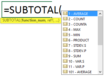
There are multiple numbers of function numbers available, but no problem; we do not need to remember all these function numbers because, while using the SUBTOTAL formula, excel will automatically show you the list of function numbers available as below.
You must be wondering why there is two function number for the same function.
- 1 – 11 function numbers should use when we want to ignore the filtered-out cells and consider the manually hidden cells.
- When we want to ignore all the hidden cells, including the ones filtered out and manually hidden cells, we should use function numbers like 101-111.
We will see a few examples to understand how the subtotal function will work for different function numbers.
How to Use SUBTOTAL Formula in Excel?
SUBTOTAL Formula in Excel is very simple and easy. Let’s understand how to use the SUBTOTAL Formula in Excel with some examples.
Example #1
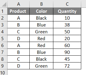
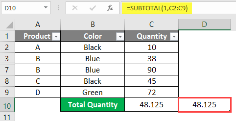
Consider a small table that has data from different categories as below.
We have a Product Category, Color category, and quantity if you observe the above table.
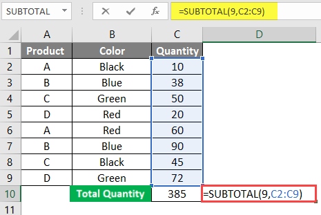
Apply the SUBTOTAL formula as below with function number 9.
After applying this formula, the result is shown below.
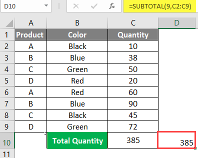
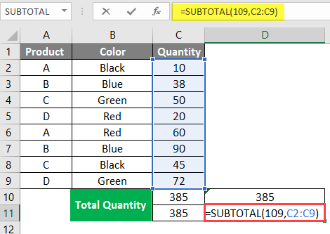
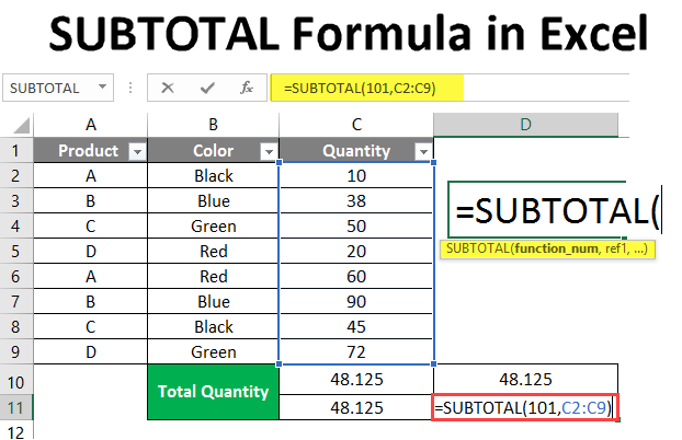
Apply the SUBTOTAL formula as below with function number 109.
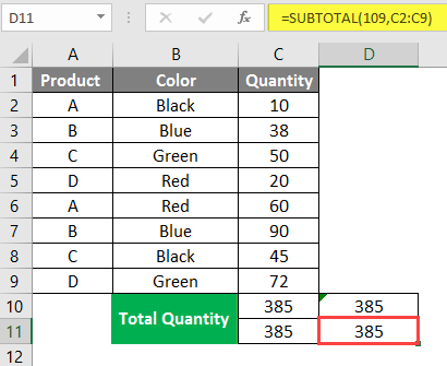
After applying the SUBTOTAL Formula, the result is shown below.
We used function numbers 9 and 109 in the formula to perform SUM in two columns. C2:C9 is the range of data that we are performing calculations.
Now, the total sum is 385 for both formulas. Hide a few rows and observe the results for both formulas.
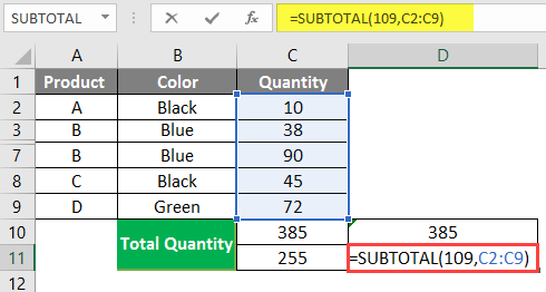
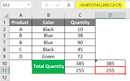
After applying the SUBTOTAL Formula, the result is shown below.
Rows from 50 to 60 are hidden; hence the results of function number 109 have changed to 255 because it does not consider the manually hidden data, whereas function number 9 total remains the same, meaning it will consider the data even though we hide it manually.
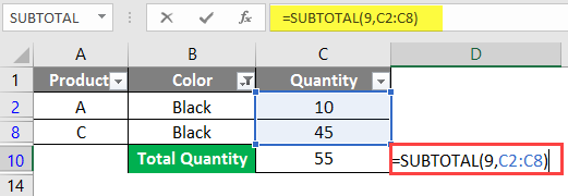
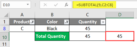
Apply filter to the data and filter only one color; the Black Color is selected here.
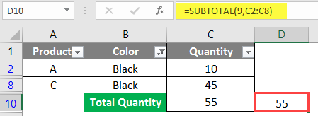
After applying the SUBTOTAL Formula, the result is as shown below.
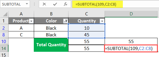
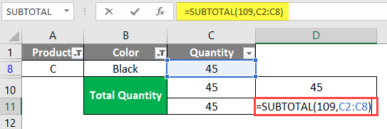
Apply the SUBTOTAL Formula as below with Function Number 109.
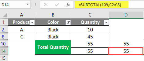
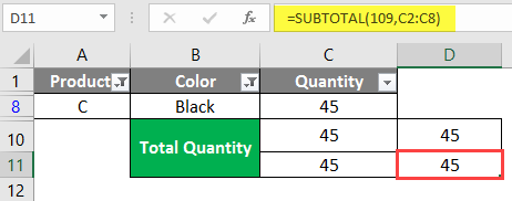
After applying the SUBTOTAL Formula, the result is as shown below.
If we observe the above screenshot, both the function numbers did not consider the quantity of filtered-out data. After you filter out the data and hide rows, both formulas will give the same results that both formulas will not consider non-visible data.
After applying the SUBTOTAL Formula, the result is as shown below.
Apply the SUBTOTAL Formula as below with Function Number 109.
After applying this formula, the result is shown below.
Example #2
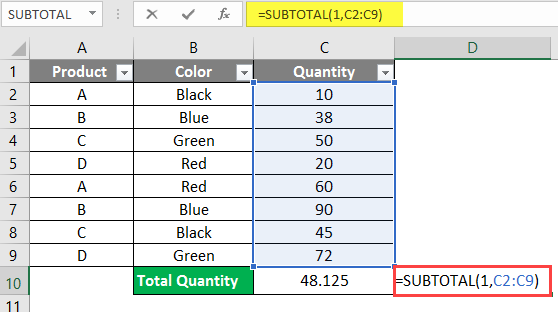
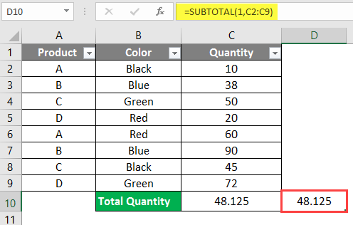
We have seen the SUM operation; now, we will perform the AVERAGE operation with the same data range. Go through the above table for the details of function numbers details. 1 and 101 are the function numbers to perform average.
After applying the SUBTOTAL Formula, the result is as shown below.
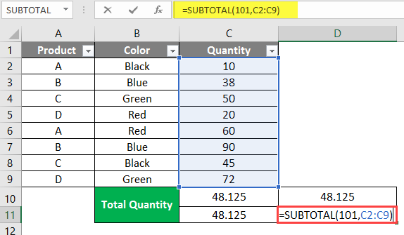
Applying the SUBTOTAL formula again with function number 109 for the next cell.
After applying the formula, the result is shown below.
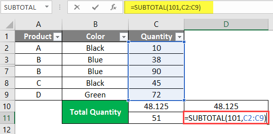
With the same SUBTOTAL Formula, we can calculate the average with the only change in Function Number.
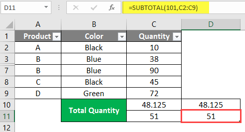
After applying the SUBTOTAL Formula, the result is as shown below.
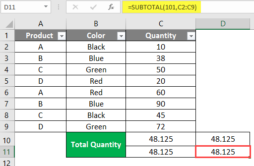
Applying the SUBTOTAL formula again with Function Number 101 for the next cell.
After applying the SUBTOTAL Formula, the result is shown below.
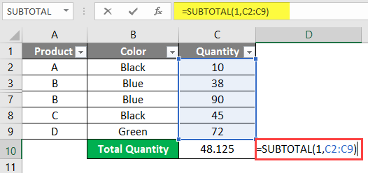
Hide a few rows; now observe the changes in the average. The average with function number 1 remains the same as still; it also considers the hidden quantity. The average with function number 101 changed because it ignores the manually hidden data. Like this, you can try the rest of the function numbers and check each functionality as the basic concept is the same; they also will work in the same way.
Example #3
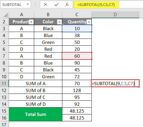
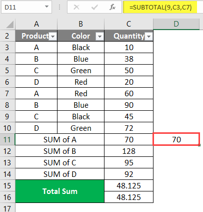
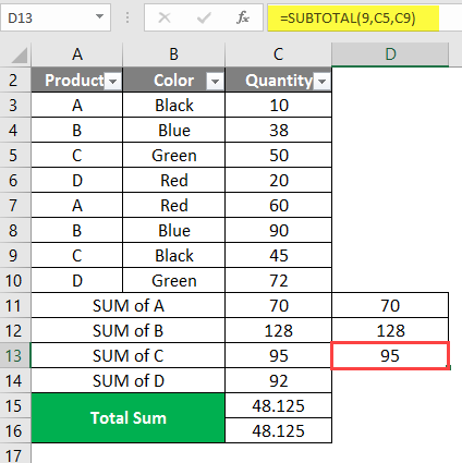
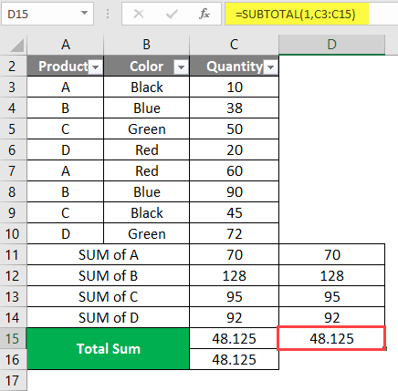
Subtotal has one more advantage: it will not consider any subtotals available in the range of data. We will see one example to understand better. Input formulas to perform SUM operation product-wise like A, B, C, and D. It doesn’t need to be product-wise; you can do it color-wise also.
After applying the SUBTOTAL Formula, the result is as shown below.
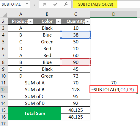
Use the SUBTOTAL formula again to check the SUM of B.
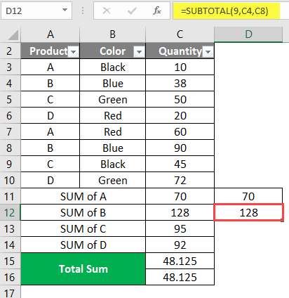
After applying the SUBTOTAL Formula, the result is as shown below.
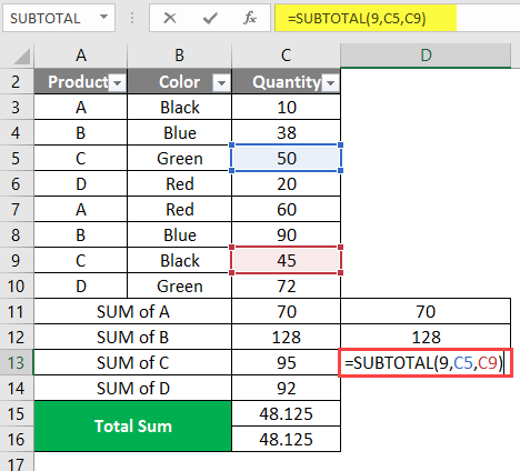
Use the SUBTOTAL formula again to check the SUM of C.
After applying the SUBTOTAL Formula, the result is as shown below.
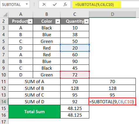
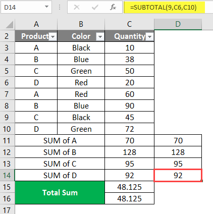
Use the SUBTOTAL formula again to check the SUM of D.
After applying the SUBTOTAL Formula, the result is as shown below.
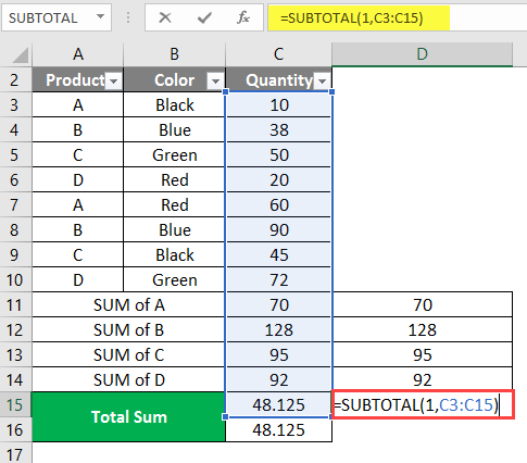
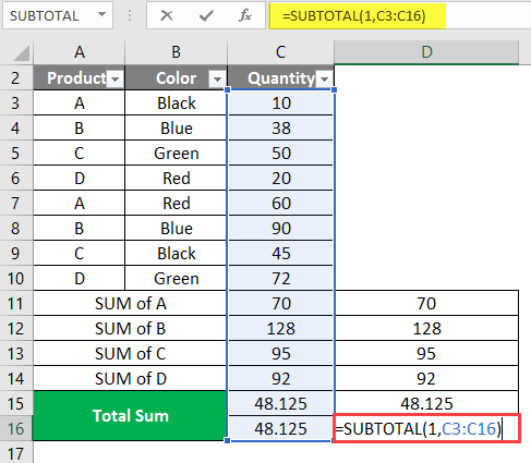
Use the SUBTOTAL formula again for the next cell.
After applying the SUBTOTAL Formula, the result is as shown below.
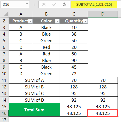
Use the SUBTOTAL formula again for the next cell.
After applying the SUBTOTAL formula, the formula displays the resulting value below.
If we observe the above screenshots, there is a sum by-product wise, and while performing the total sum, we included the category-wise totals into the total sum (cells from 36 to 48), but it will not consider that subtotals (cells from 44 to 47). So, we can calculate the subtotals between the data range without affecting the total sum value.
I hope you understand how to use the subtotal and the use of it.
Things to Remember
- While giving the function number, do not give the number out of the function number range as Excel does not predefine it; we will get an error message. We should always provide the number between 1 to 11 and 101 to 111; otherwise, it will throw the error message #value.
- While using the division operation, remember no number should be divisible by zero. That means x/0 is an incorrect format.
- If you apply the subtotal for horizontal data from A1: F1, hiding any columns will not impact the subtotal.
- While applying subtotal, if any cells do not have data or non-numeric data, the function will ignore those cells.
- Use the function numbers by understanding the functionality and use; otherwise, you might not get the correct results you expect.
Recommended Articles
This has been a guide to the SUBTOTAL Formula in Excel. Here we discuss How to Use the SUBTOTAL Formula in Excel, practical examples, and a downloadable Excel template. You can also go through our other suggested articles-

