Updated March 8, 2023
Introduction to Support Vector Machine in Machine Learning
Support vector machine in machine learning is defined as a data science algorithm that belongs to the class of supervised learning that analyses the trends and characteristics of the data set and solves problems related to classification and regression. Support vector machine is based on the learning framework of VC theory (Vapnik-Chervonenkis theory) and each of the training data points is marked as one of the 2 categories and then iteratively builds a region that will separate the data points in the space into 2 groups such that the data points in the region is well separated across the boundary with the maximum width or gap.
The setting up of different data points into respective one of the 2 categories is a non-probabilistic binary classifier. Now when a new example comes into the space, the corresponding group is predicted from the features and assigned the same group.
How Support Vector Machine Works in Machine Learning?
Support vector machine is able to generalize the characteristics that differentiate the training data that is provided to the algorithm. This is achieved by checking for a boundary that differentiates the two classes by the maximum margin. The boundary that separates the 2 classes is known as a hyperplane. Even if the name has a plane, if there are 2 features this hyperplane can be a line, in a 3-D it will be a plane, and so on. In the sample space, there is a possibility of zillions of hyperplanes but the objective in a support vector machine is to find that hyperplane through an iterative process that determines the hyperplane that has the maximum margin from all the corresponding training points and this will facilitate any new point coming in to fall into the accurate class on the basis of the features.
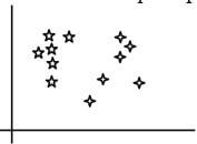
It is now time for us to know about the working of a support vector machine. There are 2 types of data and the approach in SVM towards the types of data is henceforth a bit different as well. For the first type of data, it needs to be linearly separable. Let us say that the data is spread across the sample space in the below way. For simplicity let us assume the data is a 2-D, and we will gradually move it to a 3-D as well in subsequent paragraphs.
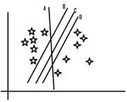
The sample space will give rise to the following lines for being the hyperplane. Let us name them A, B, C, D.
In the above graph, we see that all the hyperplanes are accurately classifying the different groups we have in the data set. But the question is which of them does that with more cleanliness. Let us take each of them one by one. Line A does the job, but 2 points are very close to the line, and even a single movement might put the model into the confusion of which is correct and what is not. Now looking at line B, we see that the 5 pointer stars are very close to that line and hence still have the risk of getting misclassified even with a slight change. With line D, the 4-pointer stars are closer and hence stand the most chance of misclassification. With this, we are left with only line C that proves to be the best of the lot. The data points that are closest to the separable line are known as the support vectors and the distance of the support vectors from the separable line determines the best hyperplane.
What did we do here?
We followed some basic rules for the most optimum separation, and they are:
- Maximum Separation: We selected the line that is able to segregate all the data points into corresponding classes and that is how we narrowed it down to A, B, C, D.
- Best Separation: Out of the lines A, B, C, D, we chose the one that has the maximum margin to classify the data points. This is that line that has the maximum width from the corresponding support vectors (The data points that are the closest).
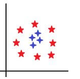
Not every time we might encounter data that is linearly separable and that is what brings us to the other type of data and that is non-linearly separable data. For this, we would need to decide the boundary as well, but do you think there can be any straight line that will be able to differentiate the below data sets.
What is more important is to look for something that is beyond a straight line, may be a circle.
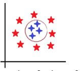
How about the below boundary?
Do we now observe that they are separated perfectly? Of course, they are much better than a line could have done. This is what is known as a kernel trick. In a kernel trick, the data is projected into a higher dimensions and then a plane is constructed so that the data points can be segregated. Some of these kernels are RBF, Sigmoid, Poly, etc. Using the respective kernel, we will be able to tune the data set to get the best hyperplane to separate the training data points again using the 2 rules seen above.
Example of Support Vector Machine in Machine Learning
Given below is the example mentioned:
SVM using the FAMOUS iris dataset.
Syntax:
import numpy as np

import matplotlib.pyplot as plt

from sklearn import svm, datasets

dfIris = datasets.load_iris()

features = dfIris.data[:, :2]
target = dfIris.target

C_grid = [1,10,100,1000]
svc = svm.SVC(kernel='linear', C=1, gamma='auto').fit(features, target)

x_low, x_high = features[:, 0].min() - 1, features[:, 0].max() + 1

y_low, y_high = features[:, 1].min() - 1, features[:, 1].max() + 1

height = (x_high / x_low)/100

xAxisGrid, yAxisGrid = np.meshgrid(np.arange(x_low, x_high, height),

np.arange(y_low, y_high, height))

plt.subplot(1, 1, 1)

predSVM = svc.predict(np.c_[xAxisGrid.ravel(), yAxisGrid.ravel()])

predSVM = predSVM.reshape(xAxisGrid.shape)

plt.contourf(xAxisGrid, yAxisGrid, predSVM, cmap=plt.cm.Paired, alpha=0.8)

plt.scatter(features[:, 0], features[:, 1], c=target, cmap=plt.cm.Paired)

plt.xlabel('Length of Sepal')

plt.ylabel('Width of Sepal')

plt.xlim(xAxisGrid.min(), xAxisGrid.max())

plt.title('Linear Kernel plot for SVM')

plt.show()

for c in C_grid:

svc = svm.SVC(kernel='rbf', C=c,gamma='auto').fit(features, target)

x_low, x_high = features[:, 0].min() - 1, features[:, 0].max() + 1

y_low, y_high = features[:, 1].min() - 1, features[:, 1].max() + 1

height = (x_high / x_low)/100

xAxisGrid, yAxisGrid = np.meshgrid(np.arange(x_low, x_high, height),

np.arange(y_low, y_high, height))

plt.subplot(1, 1, 1)

predSVM = svc.predict(np.c_[xAxisGrid.ravel(), yAxisGrid.ravel()])

predSVM = predSVM.reshape(xAxisGrid.shape)

plt.contourf(xAxisGrid, yAxisGrid, predSVM, cmap=plt.cm.Paired, alpha=0.8)

plt.scatter(features[:, 0], features[:, 1], c=target, cmap=plt.cm.Paired)

plt.xlabel('Length of Sepal')

plt.ylabel('Width of Sepal')

plt.xlim(xAxisGrid.min(), xAxisGrid.max())

plt.title('RBF Kernel for SVM with C = ' + str(c))

plt.show()
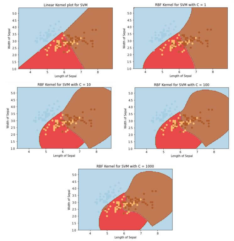
Output:
In the above plot, we see that as the kernel moves from linear to rbf, the number of data points that we were able to classify correctly increase, and we moved from 1->10->100->1000, we were able to classify it much better but only increasing the complexity.
Advantages and Disadvantages of Support Vector Machine in Machine Learning
Given below are the advantages and disadvantages mentioned:
Advantages:
- Since only the support vectors are important to determine hyperplane, this algorithm has high stability.
- Outliers don’t influence the decision of hyperplane.
- Dataset need not have predefined assumptions.
- Again, since only support vectors are involved, this algorithm is memory efficient as well.
Disadvantages:
- The training time is higher when there is a large dataset.
- In case the target class is overlapping even at a higher dimension, SVM starts to perform poorly.
- This is a black box and doesn’t provide a probability estimate, which makes it even tougher to interpret during training on what to do next.
Conclusion
With this, we come to an end to how SVM works and the intuition behind the same. It is encouraged to try experimenting with different parameters of the SVM module in python to get a deeper glimpse.
Recommended Articles
This is a guide to Support Vector Machine in Machine Learning. Here we discuss the introduction, working, example, advantages, and disadvantages. You may also have a look at the following articles to learn more –
