Updated August 11, 2023
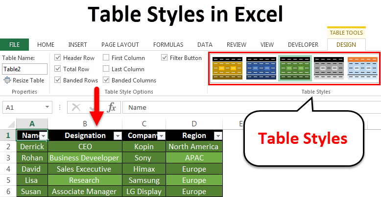
Table styles in Excel (Table of Contents)
Table Styles in Excel
In Excel, we have Table Styles which can be accessed from the Home menu ribbon’s Format As Table option under the Styles section. This gives color to the template and highlights the rows as well. We have to go in the drop-down of Format As Table option, where we will have 3 categories of Table Styles: Light Theme, Medium Theme, and Dark Theme, respectively. We can create our own customized theme for table styles, and also, we can clear the table if the purpose is fulfilled.
How to Apply Styles in Excel?
In order to apply this in to the excel table, there is a need to create an excel table. So let’s see how to create an excel table for any random data entered in the excel sheet.
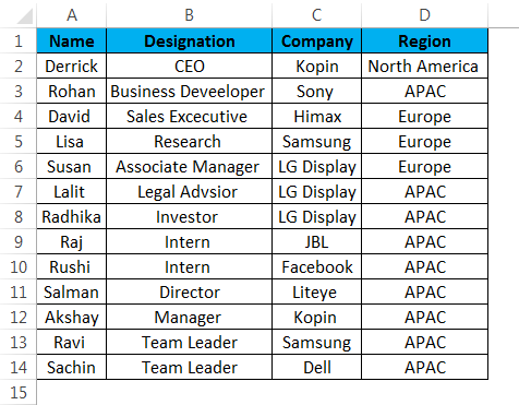
Consider the below example, where any random data is entered in the excel sheet.
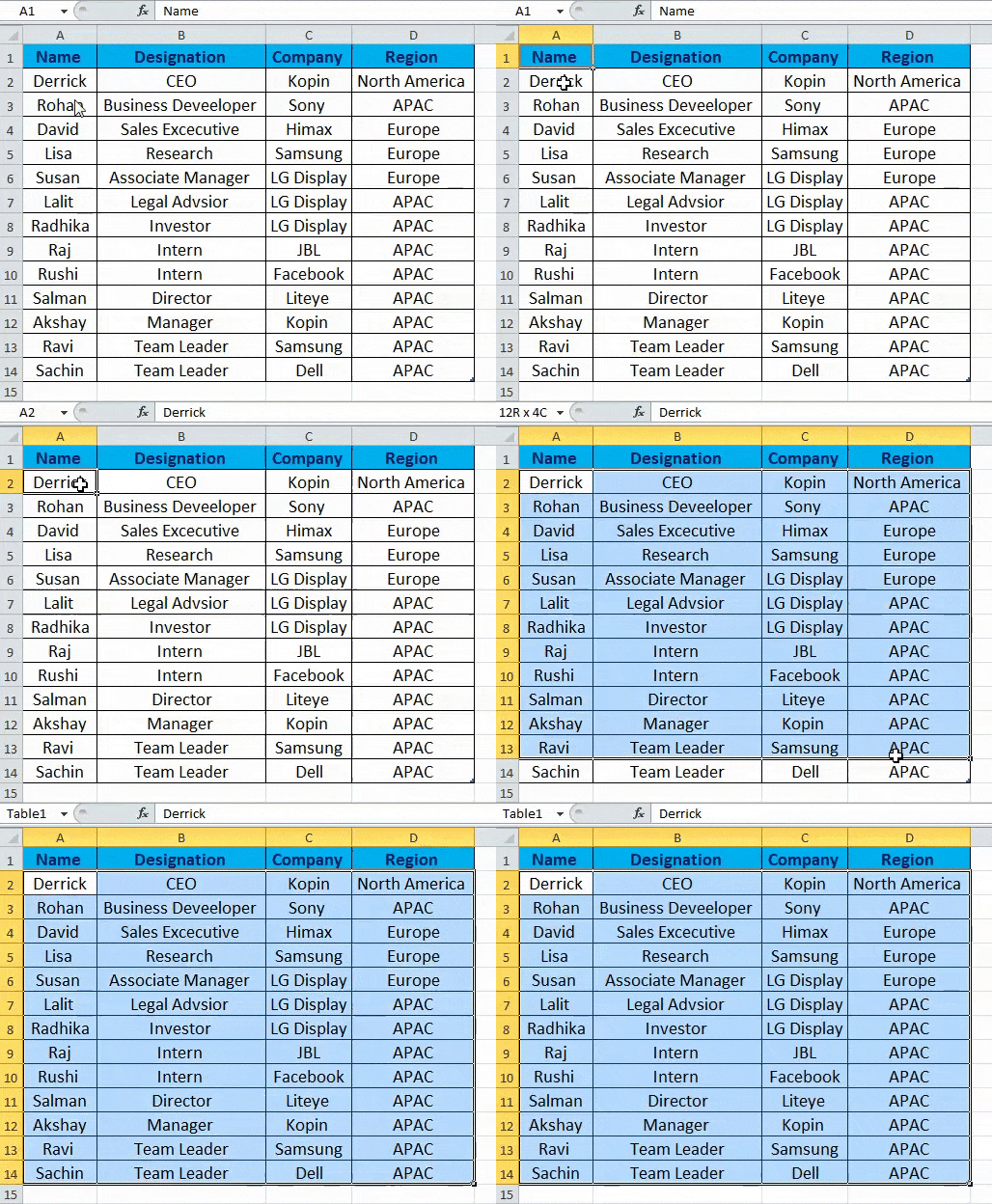
Steps to create Table entered in the sheet are as follows:
Creating a table in Excel is easy. It is easier than you think. Here we go:
Step 1 – Select the entire data in the excel sheet.
Step 2 – From the ‘Insert’ tab, select the option ‘Table,’ or else you can also press ‘Ctrl +T,’ which is a shortcut to create a table.
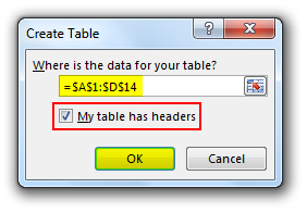
Step 3 – After selecting the table option or creating a table, you will get the ‘Create Table’ dialog; in that dialog box, click on ‘OK.’
Make sure that the ‘My table has headers’ option is ticked.
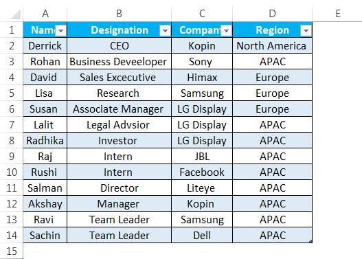
The below image shows the data entered in the tabular form.
After creating the excel table, let us see how to apply different table styles to it. In order to check different table styles, select the ‘Table Styles’ option from the ‘Design’ tab, as shown below.
The below image shows how modification could be done to your table by clicking the design tab, selecting the ‘Table Styles’ option, and selecting your preferred style.
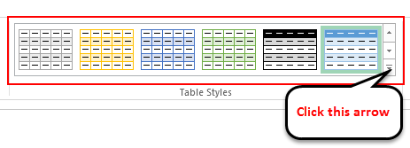
Let us explore the ‘systes’ option as mentioned in the below image. Click the arrow as highlighted in the below image.
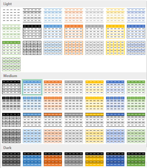
As you can see in the below image, there are more than 55 table styles available. These are grouped under the following categories:
- Light
- Medium
- Dark
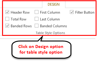
Apart from the above table styles used for formatting our excel table, we also have another ‘Table Style Options’ as shown in below.
So let us see in brief what does the above ‘Table Style Options’ mean:
- Header Row: It is used to display or hide the table headers.
- Total Row: It is used to add the total rows at the end or bottom of the excel table, along with the list of functions for each total row cell.
- Banded Rows & Banded Columns: It is used to display the alternative shading to rows or columns or both together.
- First & Last Column: Used to apply special formatting for the first and last column of the table.
Now, let us explore the above options and see the changes after applying these features to your table.
We have selected the table style from the ‘dark’ category highlighted in the below image.
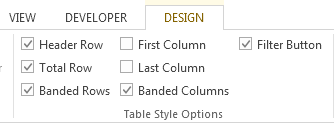
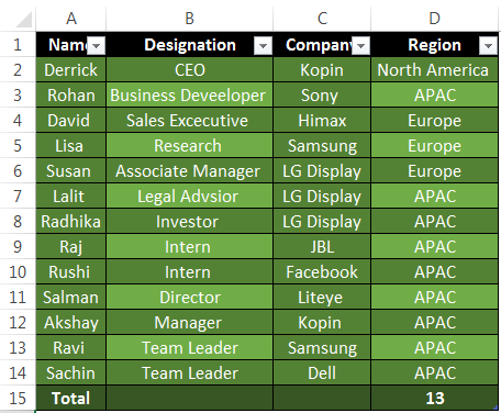
Here, we have selected Header Row, Total Row, Banded Rows, and Banded Columns.
In the below image, you can see the changes that appeared. So we can observe that shading has been applied to alternate columns after selecting the banded column option. Also, it displays the total number of rows after selecting the total row option.
Changing the default Table Style in Excel
Excel has a good feature where we can also change our default table style in excel. Follow the steps as mentioned below:
Step 1 – First, create an excel table. In this step you the default excel table will appear with default styles.
Step 2 – After preparing an excel table, click any cell from the table rather than under the ‘Design’ tab, go to ‘Table Styles’, and choose any style you prefer as your default table style.
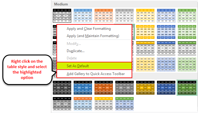
Step 3 – After selecting the particular table style according to your choice, Right-click and select the ‘Set As Default’ option. After this, your default table option is selected.
Advantages of Table Style in Excel
- Useful in cases where the user is presenting the data at any conference or presentation, and the audience should easily read it.
- Allows the user to set their preferred table style and save it as a custom table style option as well, which saves time and in case the user needs to create the excel table following the long procedure again.
Things to Remember
- In Excel versions above 2007, the table style options have added the feature as the ‘Filter button.’
- If you have manually highlighted the rows of the table or changed any formatting for the table and want to apply new styles, excel will keep the manually applied formatting in place. For this, you need to remove the existing formatting by right-clicking on the styles and selecting ‘Apply and Clear Formatting.
- Excel also allows the user to create a custom table style of the user’s choice.
- The most useful feature of this is the preview option, which allows users to preview their preferred style options.
- Also, the user can apply the table without creating the excel table by simply going to the ‘Table Tools’ tab, then on the Design option, and then selecting the ‘Convert to Range’ option.
Recommended Articles
This has been a guide to Table styles. Here we discuss the Table styles in Excel and how to use the Table styles in Excel along with practical examples and a downloadable excel template. You can also go through our other suggested articles –
